
Statistical Confidence
Statistical Confidence Can Help Pinpoint Value.
Many questions have arisen concerning the reliability of valuations using the Direct Market Data Method (DMDM). Rand Curtiss shows how to use statistical techniques to answer them with confidence.
Many questions have arisen concerning the reliability of valuations using the Direct Market Data Method (DMDM). This article shows how to use statistical techniques to answer them with confidence.
My statistics professor warned me that asking “why” in his class would cause trouble, because the answers involved heavy-duty higher mathematics. I heeded that warning, and pass it along to you. Some of what I say—all of it clearly labeled—must be accepted on mathematical faith. If you would like to explore the mathematics more deeply, please read Jay Abrams’ excellent Quantitative Business Valuation (McGraw Hill: 2001), especially Chapter 2.
 I am indebted to Jay for his technical review of this article, and for contributing the picture referenced below. One more disclaimer: the DMDM is not a panacea. Even if all of the technical statistical issues addressed herein are satisfactorily addressed, there are always concerns about the accuracy of the underlying transaction data, their validity, and pertinence. As an example, the market for medical practices has undergone revolutionary changes in the last decade, which have fundamentally affected their valuations. One would be hard-pressed to justify the use of practice transaction data more than ten years old (or maybe even more than five years old).
One of the reviewers of this article made a very good point: “An analogy might be the use of a database of residential real estate transactions for ranch style homes in an entire state. Such data might include price per square foot, price per bedroom, price per square foot of land, and so forth. No one would agree to have their (ranch) home appraised based on reported transactions from any real estate market other than the specific one within which their property was located, and from within a very tight time frame. Lacking an understanding of this data challenge, the unwary appraiser can use elegant statistical machinery and still be in error because of the old adage ‘garbage in, garbage out.”‘
The Problem
We are valuing a business using price/sales ratio (PSR) data from the IBA Database and/or other sources. We have to come up with a single number, or point estimate, for the PSR to apply to our subject business. There are ten usable observations after eliminating outliers and transactions far larger/smaller than our subject (The latter comports with the size effect.). Assume that the mean PSR is 1.1 times sales and the standard deviation is 0.3 times sales. The mean is the simple average of all of the transaction PSR’s (their total divided by the number of observations). The standard deviation is a measure of how variable the PSR’s are. It is computed as the square root of the sum of the squared differences between each sample PSR and the mean sample PSR, divided by the number of observations. Excel and other spreadsheets calculate sample sizes, means, and standard deviations easily.
We are considering whether and how to use this PSR data based on its reliability (We might adjust the subject’s PSR depending on our assessment of the relative attractiveness and riskiness of the subject. That process is not presented in this article for reasons of brevity and to keep the focus on statistical, rather than appraisal technique. Ray Miles has published several papers and monographs on that subject.). What we need to know is: how reliable is our estimate of a PSR, based on our sample of 10 data points, its mean of 1.1 and its standard deviation of 0.3? Together, these are called the sample statistics.
This simple question has profound appraisal and mathematical implications. The appraisal issues involve the relationship among different ways of expressing value: point estimate, interval estimate, and probability distribution. The mathematical implications form the foundation of the subject of statistical analysis.
Appraisal Implications
We are used to thinking about value as a point estimate, or an “amount certain.” Almost all economic transactions involve point estimates: e.g., gasoline costs $1.39 per gallon as of this writing. We could not do business without accepting point estimate prices; otherwise we would be forever haggling (as is done in other cultures).
Higher-level transactions like commercial real estate leases, professional athlete contracts, and mergers and acquisitions often include contingent (uncertain) amounts, such as rents partially based on sales, bonuses for individual performance , and payouts based on future profits. These contingencies introduce the concept of risk (uncertainty) to be shared by the contractual parties. In each case, specific risks are identified and quantified.
Business appraisers sometimes introduce risk when we are asked to provide value ranges. Let’s call these “interval estimates.” We might conclude that a business is “worth from $1.2 to $1.6 million depending on (specific assumptions).” An interval estimate usually implicitly assumes that all values in the range are equally probable.
The next level of sophistication recognizes that some values in the range are more likely than others. We might portray this in an income approach-based valuation in which we develop most likely, worst- and best-case scenarios. Here the probabilities are not quantified, but it is implicit that the most likely scenario has a higher probability than the other two. This is where the DMDM comes in: at its core, it is about ranges of value and relative likelihoods. The highest level of sophistication is to develop probability weights for each outcome. The probabilities are the relative likelihoods of each one. We could then graph the outcomes and their probabilities, forming what is called a probability distribution.
Statistical Implications
Back to our valuation example, we do not know either the actual mean or actual standard deviation of the PSR. In statistical terminology, the term ”population” is used when discussing the unknown actual statistics (mean and standard deviation). They are unknown because we cannot obtain all of them. The sample mean is 1.1, and the sample standard deviation is 0.3. Note the italicized terms, which continue for emphasis in this article, because it is very easy to confuse sample and population statistics. Remember: we know the sample statistics: we use them to make inferences about the unknown population statistics. The question of reliability is really a quality assessment of our inferences.
We cannot determine the population mean or standard deviation. To do so, we would need to have information on every single transaction in the population, which is obviously impossible (since not every transaction is disclosed, and even if they were, the cost of getting them and being sure of them would be prohibitive). We want to draw statistical conclusions about the population mean PSR based on the sample statistics: mean = 1.1, standard deviation = 0.3, sample size = 10. More rigorously, we have a point estimate of its average (the sample mean) and a point estimate of its uncertainty (the sample standard deviation), which depend entirely on the magnitudes of our (sample of) 10 observations. This is where statistical analysis begins. But first, we must accept three articles of faith:
First: we assume that each sample observation was randomly selected from the population of actual transactions; i.e. that the sample observations have no biases. This is not hard to swallow. Our elimination of outliers might violate randomness if we had a very small sample (say five or less) to start with, because it would be very hard to determine outliers, particularly if the individually observed PSR’s varied widely (Is there an outlier in a sample with values of 1.0, 1.1, 1.1, 1.2 and 1.3? You make the call.)
The protection against this would be to complete our analysis including all suspected outliers and see how much our conclusion changed. A second violation could be that the data points were not collected randomly, but since IBA and others cast wide nets in search of transaction (population) data, this does not seem to be a big risk. Ray Miles has addressed other possible violations, including geographic location and date of sale, in other IBA publications and his monographs on the DMDM, which he developed.
Second: we assume that the sample observations (the guideline transactions) were drawn from a statistically large and “normal” population that, if graphed, would look like the “bell curve,” symmetric about the mean (which would also be the most frequent, or mode value and also the median value). This is harder to accept, but is based on the fact that with enough transactions (large sample size), individual biases (like imperfect information or coercion which influenced PSR’s up or down) average out. Some people have questioned whether the assumption of statistical normality holds, given that rates of return cannot be below 0% but can be potentially infinite. This is a valid advanced criticism, which we simply cannot address in this article.
Third: in a case like ours, where the population (not the sample) mean and standard deviation are unknown and the first two articles of faith are valid, the probability distribution relevant to our reliability questions is “(Student’s) t” distribution, a shorter and flatter variation of the bell curve which is symmetric about the mean, and has a standard deviation (both of which we will use in our analysis). This is the hardest article to accept, and all I can tell you about it is that Student was a famous mathematician and my statistics professor (remember him?) told us not to ask “why” just before he told us to use Student’s t distribution. It also turns out that for sample sizes of 30 or more, you can use either the t or normal distribution, because they are virtually the same).
Preview of Coming Attractions
A picture is indeed worth a thousand words. This one is reprinted from Jay Abrams’ book, cited above, and appears on page 35 as Figure 2-2.
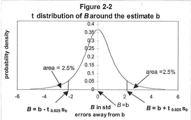
The picture is of a t curve. It looks like the bell curve. (No asking why!). The vertical axis is the probability. The horizontal axis is the PSR. The two vertical lines (B = b ± t o.02s sb) are the Lower (left) and Upper (right) Confidence Limits. The line segment from the Lower to the Upper Confidence Limit is the “Confidence Interval,” and the central section of the curve above the Confidence Interval is the “Confidence Region.” The two outlying sections under the curve are the “Critical Regions.” In the picture, the “B” is the unknown but inferred population mean PSR and the “b” is the sample mean PSR. This completes the picture, but what does it mean? Based on the articles of faith, our sample data, and our picture, we have constructed a t probability distribution. Assume it has our sample mean of 1.1.
What we want to know is: how reliable is this estimate of the population mean PSR? More formally, we are hypothesizing that the population mean PSR is equal to 1.1 based on the sample statistics: mean 1.1, standard deviation 0.3, size 10, and the three articles of faith. Enter the confidence interval. Using this information, we can construct a range, or interval estimate, of the population mean PSR and then a corresponding t distribution. This information will let us make statements like “We are 95% confident that the population mean PSR falls within the range of 1.1 plus or minus (some number to be determined).” That is a very useful reliability statement!
Setting up the Math
We now tie everything together by attaching numbers to the confidence limits. But first, we have to make one more decision, which may seem trivial, but is very important. That decision is: how confident do we want to be? The obvious answer is 100%, but we cannot get there because we cannot get all of the data, as described above. If we had it all, this entire exercise would be unnecessary; we would just compute the population mean PSR and be done. Pragmatically, how close to 100% need we be? Anything less than 90% sounds too low on the merits. Let’s compromise and use 95%, which is a generally acceptable level of confidence (I will abstract from Daubert considerations; you might select 99%, 99.9%, 99.995% or whatever, but as will be shown below, as the confidence level [95%, 99%, etc.] rises, the confidence interval gets wider, which means there is a bigger range around our estimate.). Saying that we are 99.995% confident that the population mean PSR is between -5 and +5 doesn’t really help us (In the words of Bart Simpson, “Doh!”)!
We need a narrower range, or confidence limit. Regardless of the confidence level selected, the procedure is the same. You need either t tables from a statistics book or the mathematical knowledge to build the appropriate spreadsheet.
What our “95% confidence level” means is that we are statistically 95% confident (sure that 95% of the time) our confidence interval (the range of PSR’s between the lower and upper limits) will include the (unknowable) population mean PSR. Or, 95% of the time, the population mean PSR will be in our confidence interval of 1.1 plus or minus some number.
This is very helpful! We have gone from a sample average PSR of 1.1, which sort of floats out there in space to being able to say we are 95% sure that the population mean PSR is within our confidence interval, which is 1.1 plus or minus some number (which we are about to calculate).
Doing the Math
For brevity in our formula, define:
m = sample mean = 1.1
s =sample standard deviation= 0.3
n = sample size = 10
c = confidence level= 95% or 0.95
t = the t statistic, which depends on n and c
There are two more conceptual points. First, looking again at the picture, the confidence interval and the confidence region are the line and area under the curve in the center between the upper and lower confidence limits.
There are two critical regions, one to the right and one to the left, outside the confidence region. Since the t distribution is symmetric, the two critical regions are of equal size. The second point is that the confidence level tells us how big the confidence region is; that is, how much of the area under the curve is represented by the confidence region. The 95% confidence level means that the confidence region includes 95% of the area under the curve.
The two critical regions together include the other 5%. Since they are of equal size, each includes 2.5% of the area. The lower critical region plus the confidence region contains 97.5% of the area.
Let’s define one more variable:
v = confidence level + [1/2 * (100%- confidence level)]
= 95% +[1/2 * (100%- 95%)] = 97.5% = 0.975
We can see that v is the upper confidence limit.
We calculate or look up the t statistic using the sample of size n= 10 and the upper confidence limit (v = 0.975). The table tells us that t = 2.228.
The formula for the confidence interval is:
Confidence interval= me ± (t * s / √ n ) …. √ n is the square root of n
= 1.1 ± (2.228 * 0.3 / √ =10) = 1.1 ± 0.21
= from 0.9 to 1.3, rounded
We can now state with 95% confidence that the population mean PSR is within 1.1 ± 0.2, or from 0.9 to 1.3. This is a pretty reasonable, comfortable spread for appraisers to use as a range of PSRs.
The higher the confidence level is, the wider the confidence interval will be, the smaller the critical regions will be, and the larger the resulting plus or minus number and range will be.
If we chose a 99% confidence level, the corresponding t statistic for n = 10, v = 0.995 is 3.169. The confidence interval computes to 1.1 ± 0.3, or from 0.8 to 1.4. We are 99% sure that the population mean PSR is within this range. We are more confident (99% as op posed to 95%), but the range is wider. This makes sense; we are surer of being in the range, but it is bigger.
If we chose an 80% confidence level, the corresponding t statistic for n = 10, v = 0.90 is 1.372. The confidence interval computes to 1.1 ± 0.1, or from 1.0 to 1.2. We are 80% sure that the population mean PSR is within this range. We are less confident (80% as opposed to 95%), but the range is narrower. This makes sense; we are less sure of being in the range, but it is narrower.
Another important point is that the more observations we have (as n increases), the confidence interval becomes narrower, which means that we gain a more confident estimate of the unknown population mean PSR. Back at the 95% confidence level, for n=10 the t statistic was 2.228. For n=l1 the t statistic drops to 2.201. At n=20 it drops to 2.086. At n=60 it drops to 2.000. For an infinite sample size, it drops to 1.96. Going the other way, with smaller samples, at n =5 the t statistic rises to 2.571. Use of the DMDM for samples of less than n=6 is not recommended.
This is because the t statistic rises exponentially. With a sample of n=2 it is 4.303 and with a sample of n=1 it is 12.71. The t statistics of this magnitude yield such wide PSR ranges that they are useless. Would you quote a PSR range of from 0 to 20?
The last paragraph shows that sample size increases do not yield great benefits once there are ten data points. In other words, you are on pretty strong statistical ground with a sample size of ten or more. From five to ten, you are statistically okay, but getting wider ranges that make the results less useful. Samples of less than five are statistically unsafe.
Also note that the confidence interval is directly related to the sample standard deviation (s) in addition to sample size (n). A low s will lead to a narrower confidence interval, which is helpful statistically, not to mention psychologically. You would be happy to quote an (estimated population) PSR range of 0.9 to 1.3 with 95% certainty, as developed in the example above.
These last two points bear emphasis. They mean that “good quality” data, meaning data with a low standard deviation (s, or dispersion) can mitigate lack of “quantity” of data, (n, and the sample size). The next table shows the confidence intervals calculated for different assumptions about quality (s) and quantity (n), varying only one at a time, with everything else held constant (mean=l.1, confidence level=0.95):
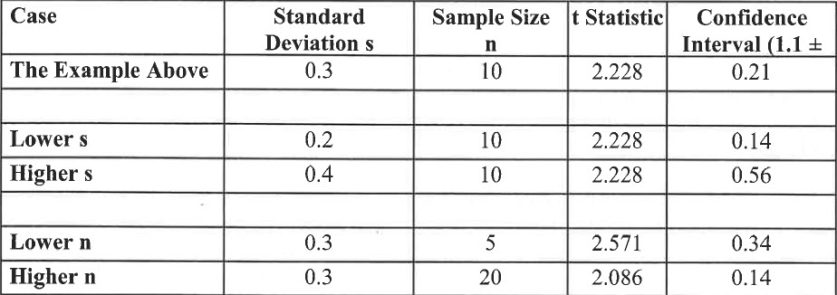
“Better quality” data (with a lower standard deviation) lead to a narrower confidence interval, and “poorer quality” data (with a higher standard deviation) lead to a wider confidence interval. More data (larger sample size) leads to a narrower confidence interval, and less data (smaller sample size) leads to a wider one. Putting it all together, you might have few data points (a sample size less than 10), which is shaky on statistical grounds because the t statistic will be bigger and n will be smaller, but low variability (standard deviation) could offset this.
Final Points
IBA Members and ADAM subscribers may access the IBA Market Database for free and get data electronically for use in spreadsheet programs, which facilitate calculations of sample sizes, means, and standard deviations as preludes to computing t statistics and confidence intervals. This article has shown how to do this and then how to use them to make reliability statements about your conclusions.
Those more statistically inclined can, remembering those same warnings, use t statistics to develop percentiles. For example, harking back to our case study, to develop the 95th and 5th percentiles, use the 90% confidence level (remembering from the picture that half of the uncertainty will be in each of the two critical regions, so with c = 0.90, v = 0.95).
Hyper technically, this technique treats the variability of the sample data points (via the sample standard deviation) more rigorously than the analysis in the previous paragraph. On the other hand, the incremental technical sophistication may not be worth the additional time, cost and complexity it creates for both you and your readers. Do you really want them to ask you “Why?”
Rand M. Curtiss, FIBA, MCBA, is President of Loveman-Curtiss, Inc. in Cleveland, Ohio, and Chair of the American Business Appraisers National Network.
This article originally appeared in the Spring 2003 Issue of Business Appraisal Practice (BAP). Visit www.Go-IBA.org
Related posts
-

Squashing Small Business
-

Einstein and Valuation: It’s All Relative!
-

Being Effective and Efficient
-

Scoping an Engagement: Questions to Consider Before Any Appraisal, Part II
-

Scoping an Engagement: Questions to Consider Before Any Appraisal
-

Investment Profiles and Valuation Discounts
-

Which Discount and/or Premium Applies?
-

Five Key Questions to Determine an Appraisal’s Scope and Fee
