
An Overview of Methods for Estimating Lost Revenues in Economic Damages
Forecasting “But-For” Revenue for Lost Profits
In this article, the author provides a brief discussion of each major approach considered in an economic damages engagement and then discusses circumstances in which multivariate analysis could provide the greatest benefit in formulating a comprehensive damage model.

Economic damages[1] can be defined as the difference between what an alleged impaired subject company would have performed but for the consequences of an alleged tort. Torts may vary from intellectual property infringements to breach of contracts to misrepresentation of financial data. In each instance, however, the plaintiff typically alleges that but for the defendant’s wrongful act or infringement of a right, the plaintiff entity would have performed better. The difference between this hypothetical ‘but-for’ (that is, a world where the alleged tort does not occur) and that of the actual history (that is, a world where the alleged tort did occur) are commonly defined as economic damages. As such, the role of the damages expert is—to a large degree—one of creating revisionist history, that is, mapping out the expected economic performance a subject company would have achieved “but for” the alleged tort. This involves estimating “but-for” revenues, expenses, and quantities.
The appropriate methods damages experts utilize to generate these estimated profits vary depending upon the specific circumstances of each case. Commonly utilized methods include before-and-after, market share, industry average, and expect value approaches. In the following sections I provide a brief discussion of each approach and then discuss circumstances in which multivariate analysis could provide the greatest benefit in formulating a comprehensive damage model. I also outline how a valuation analyst might utilize the data.
Before-and-After Approach
Plaintiff’s attorneys tend to infer a before-and-after approach within the complaint of most cases seeking economic damages. Unlike damages experts who should provide the court with an impartial analysis of the factors contributing to potential damages, attorneys are advocates for their clients. Subsequently, it is common for a plaintiff’s attorney to present the world in a very simplistic black and white image, highlighting the economic performance of their client before and after an alleged tort and attributing the cause of any and all negative economic consequences experienced by the subject company after the alleged tort exclusively on the alleged tort itself. This approach is far from comprehensive but proves attractive in both its ability to provide a parsimonious methodology to one’s audience and by allowing the plaintiff’s attorney to infer prima facie evidence that damages did indeed occur as a result of the tort.
The weaknesses of this approach should be evident to any thoughtful observer.. By attributing all negative economic performance to that of the alleged tort, the analyst must assume that all factors but for the alleged tort remained constant in both periods prior to and after the alleged harm. This is rarely the case. Other factors may have contributed to the drop in economic performance prior to the alleged wrong-doing. Assume the subject company is an airline company.. Further assume the tort (say, a breach of contract) took place on September 10, 2001. Declining sales are observed from September 11, 2001 onward for a sustained period of time. Clearly, the before and after approach would be ineffective in capturing the effect of 9/11 on the subject company’s sales, and to ignore this event would be inappropriate. Given that damages calculations involve isolating the incremental impact affiliated with an alleged tort, the before-and-after approach is usually an inappropriate (or incomplete) method for providing the court with any useful information.
Market Share Approach
Damages experts may also use a market share approach to account for possible macroeconomic factors that may have impacted and hence affected the economic performance of the subject company after the alleged tort. In a market share approach, the expert examines the market share held by the subject company before and after an alleged tort and attributes any drop in expected market share to the tort itself. Unlike the before-and-after approach, the market share approach makes the claim that macroeconomic factors have been taken into consideration for events such as a rise in interest rates or drop in gasoline prices that impact the market as a whole. The weakness of this approach is less evident, but still exists. The market share approach assumes the impact of macroeconomic factors is experienced uniformly across all competitors. While macroeconomic factors may have a general effect on all of the subject company’s competitors, it is unlikely that the effect on all of the competitors, including the subject company, will be equal. Assume the subject company is a manufacturer of automobiles. While a rise in petroleum prices may have an adverse impact on the sale of all automotive vehicles as a whole, it is unlikely that that impact would be uniform among the competitors in a similar market. While sport utility vehicles may experience a drop in sales as a market segment overall, the extent to which different models experience that drop may vary, depending upon their fuel efficiency standards. In the end, each of these influencing factors would still need to be accounted for when deriving the “but-for” scenario.
Yardstick Approach
Similar to the market share approach, the industry average (or yardstick) approach attempts to account for the macroeconomic factors that may influence sales and are unrelated to the alleged tort. In this approach, the damages expert assumes that the subject company would have performed similar to its competitors, taking into account that some adjustments may be made by looking at the standing of the subject company relative to its peers prior to the alleged tort. For example, had the subject company consistently performed five basis points below its peers, the economic expert could then incorporate this historical information in the industry average approach when forecasting future sales for the subject company. That is, the expert would make the assumption that the subject company would continue to advance five basis points below the industry average.
The advantage to this approach is that, like the before-and-after and market share approaches, it is intuitive and easy to follow. Moreover, like the market approach, it seeks to incorporate other factors that may have precipitated the drop in economic performance other than the alleged tort, allowing the damages expert to possibly isolate the incremental impact of the alleged tort.
The weakness of this approach is that it forces the damages expert to make the assumption that the subject company’s performance relative to its peer group will remain constant moving forward. This assumption may not hold and is not easily tested. The focus often becomes persuading the trier of fact (that is, the judge or jury) that the selected peer group contains appropriate comparables relative to the subject company. Nevertheless, even with appropriate comparable companies, the analysis is unable to account for different macroeconomic factors influencing companies within the group differently. The damages expert must make the assumption that the variations in performance among the peer companies are made moot by looking at the group as whole. Again, this may or may not be a valid assumption based on the specifics of the case.
Expected Value Approach
The expected value approach is a combination of both the before-and-after approach, which utilizes the subject company’s historical information during the unimpaired period, and the market and industry average approaches; these later approaches rely on comparable performance figures. Utilizing the subject company’s historical information is commonly used in these engagements, because the use of the historic data removes the burden of evaluating and defending comparable companies and establishing their relative responses to macroeconomic factors. However, this difficulty is not removed so much as ignored. Instead of basing the hypothetical ‘but-for’ on the experience of alleged unimpaired comparable companies, in the expected value approach one typically uses the subject company’s historical unimpaired information as the basis for determining the ‘but-for’ world.
The expected value approach performs the same basic analysis as the before-and-after approach, but does so with an extended time frame so that more historical data is used to create the before scenario. It is common for damages experts to take five years’ worth of historical data and calculate the compound annual growth rate of sales during the unimpaired period. The five-year period is chosen because it is assumed to capture a full business cycle, which may or may not be the case for a particular subject company or industry. As such, the arbitrary use of the five years of historical data may or may not be grounded in empirical reasoning. Some valuation analysts, and hence damages experts, may use a weighting system, whereby the last two years of the historical five-year year-over-year growth rates are subjectively weighted more heavily than earlier data.
There are two main difficulties to this approach. First, using a descriptive statistic to estimate future growth may or may not be appropriate; the assumption requires appropriate testing. And testing the degree of confidence for point estimates is impossible when they are based on a subjective weighting or on a demarcation point.
To show the importance of testing, let’s illustrate the point with an example. Assume an economist runs a trending analysis on historical sales prior to the alleged tort. A trending analysis can be conducted in Microsoft Excel by simply typing in two or more numbers in consecutive cells, highlighting them and dragging the cursor down. Excel will calculate the next number in the sequence. A respected academic economist I encountered did this exact exercise in a damages report I was asked to review. What he reported from this exercise were the expected values of the sequence moving forward. He concluded that the difference between the expected value and the actual value represented the incremental damage associated with the alleged tort. What he had done was provide the reader with a point estimate. The problem was that doing just that avoided or neglected to provide the reader with an interval estimate around his point estimate. This basic trending exercise, as the one I described in Excel, is ultimately a regression. In this case, the damages expert was running a regression of sales on time, or a trend. When you use the regression analysis function in Excel software, Excel will produce an equation that results in the same point estimates. The advantage of using the regression analysis toolpak, however, is that the results provide the standard errors of the coefficients, which allows the researcher to calculate the confidence intervals (presumably 95 percent confidence intervals) around the resulting point estimate.
In that case mentioned above, the actual sales of the alleged impaired subject company were within the confidence interval generated by a hypothesis of no damage. This means that the plaintiff’s expert’s own damages model suggested that no damages had taken place at all, or that the damage model proposed by the plaintiff’s damages expert was grossly inadequate in actually isolating out the alleged incremental impact of the subject company’s sales as a result of the alleged tort.
A second shortcoming of utilizing one descriptive statistic is that it ignores factors independent of the alleged tort which may have changed the economic environment the subject company faces. When you ignore these factors in your damage model, you are effectively assuming that all of macroeconomic factors had been held constant but for the alleged tort. This is rarely the case, if ever. The only solution to this is to control these factors. Applied multivariate regression allows the researcher to control for other factors impacting economic performance. When the researcher has at his disposal sufficient historical information, regression analysis may be an appropriate and useful technique for identifying and isolating incremental damages a subject company suffered as a result of an alleged tort.
Expected Value Approach: Regression Analysis
An appropriate expected value approach should attempt to control for all other factors impacting sales independent of the alleged tort. It should also be testable. Multivariate regression analysis allows experts to meet both of these conditions. Some attorneys are hesitant to employ damages experts who utilize this methodology in that they may question the jury’s ability to evaluate its methods, reliability, power, and application. To address this concern, I provide a brief tutorial for an audience who are less familiar with regression analysis engaged in commercial litigation on the use of regression analysis in identifying economic damages.
The construction of a regression model involves first determining the variable one seeks to estimate—typically, this variable is the subject company’s sales. This is called the dependent variable for its expected value is dependent upon the external variables that influence its expected outcome. Interest rates, for example, may influence the sale of automobiles. Additional independent variables that might influence automotive sales include disposable income or gasoline prices. The regression model therefore is made up of a dependent or endogenous variable (in this case automotive sales) that is influenced by various possible independent or exogenous variables (such as interest rates, gasoline prices, and disposable income). The relationship between the independent variables and the dependent variables are identified via the slope, or beta, coefficient of each independent variable. One can illustrate the relationship between two variables in a scatter plot, where the automotive sales are plotted on the y-axis and disposable income on the x-axis. Looking at a scatter plot, one might note positive correlation visually between these two variables, that is, as disposable income rises, automotive sales rise as well. A regression analysis seeks to transform that visual relationship into an equation. It does this by finding the line that, if laid upon the scatter plot of points, provides the best fit. The line represents the expected value of automotive sales, where the slope of the disposable income variable represents the incremental increase in sales one could expect from a change in that variable. Excel users and practitioners will note that the expected value will deviate at times from the actual sale plotted in the scatter plot. That deviation represents the error term of the model. The best fit line is that which minimizes the error term for the model. Given that the error term can be both positive and negative, the regression model squares them first to remove their sign. Hence, a common method of regression analysis is to conduct what is called an Ordinary Least Squares (OLS) model that seeks to minimize the square of the error terms.
Regression analysis allows a researcher to control for multiple variables. The output from the software used to run the regression analysis will vary but all will look similar. Following is the output from Stata, for example, where revenue was regressed on both a time trend and a time trend squared.[2]
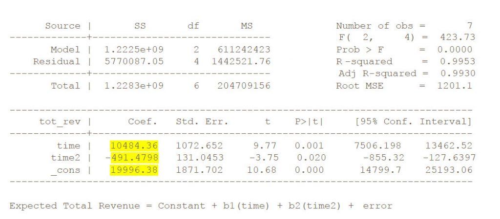
The way to read this output is as follows: expected revenue equals $19,996.38 + $10,484 (time) – $491.48 (time2). In other words, sales are expected to grow by approximately $10,484 each time interval (usually a year or a quarter) and will do so at a decreasing pace. These figures are taken from the coefficients or betas noted above in the output. Each future point in time is the point estimate derived from the model. Moreover, we know that 99.3 percent of the variation in the dependent variable, revenue, can be explained by the variation in the independent variables by observing the adjusted R-square figure. Further, we know that the independent variables time and time2 are found to be statistically significant, by looking at the figure under P>|t|, which can be interpreted as 1 – X, where X is the level of confidence one has in rejecting the hypothesis that the coefficients are not dissimilar to zero. And finally, the standard errors allow one to calculate the corresponding confidence intervals for each point estimate.
Conclusion
Each of the commonly accepted approaches typically utilized by damages experts hold advantages and disadvantages in determining the incremental impact, if any, an alleged tort had on the plaintiff’s economic performance. Multivariate regression analysis is commonly ignored by damages experts given attorneys often fear that it will be misunderstood or viewed as speculative by the juries. With a little effort, the jury or judge can be taught the underlying concept of regression analysis thereby demystifying it for them and allowing them to see that it may well serve as a superior means to isolating the incremental impact of the alleged tort, while allowing the researcher to test the accuracy of his results in a way that simply cannot be done with more traditional approaches.
[1] In particular, consequential damages.
[2] The reason one would include time squared as an independent variable is that time is thought to have a non-linear relationship with the dependent variable in this case. For example, the regression output above tells us that while expected revenue increases with time, it does so as a decreasing pace.
Richard Eichmann is based in San Francisco and Los Angeles and serves as Vice President in NERA’s Intellectual Property and Securities and Finance Practices. He has expertise in damages modeling, business valuation, econometrics, statistics, sampling, and survey research methods. He excels at drawing meaningful conclusions from large disparate datasets. His quantitative skill set has been applied in the calculation of economics damages in commercial litigation in a variety of industries, including the automotive, airline, credit card, financial, energy, gaming, and pharmaceutical.
Mr. Eichmann can be reached at (415) 291-1033 or by e-mail at Richard.Eichmann@nera.com.
Related posts
-

From Forecast to Flawed Assumptions and a Speculative Basis
-

Legal Update: March 2025
-

Accounting Expert Witness Reliably Calculates the Quantum of Monetary Harm
-

The Difference Between Lost Wages and Lost Income Analyses
-

Daedalus Blue, LLC v. MicroStrategy, Inc.
-

The Power of Artificial Intelligence and Machine Learning
-

Valuing Lost Profits of a License Agreement
-

Lost Business Profit Damages Claims
