Terminal Value

The Problem with Exit Multiples

Most of an Income Approach-based valuation is frequently in the terminal value. Thus, an Income Approach-based valuation that relies on an exit multiple to arrive at a terminal value is essentially a Market Approach-based valuation in disguise. Many practitioners do not use an exit multiple to arrive at a terminal value for this reason. Nevertheless, numerous practitioners prefer to use an exit multiple. The basis is straight-forward: the goal is to arrive at a value of the business at the end of the discrete projection period and a hypothetical sale at that time is likely to be based on a multiple of earnings. This article addresses some problems that must be addressed when trying to identify a reliable exit multiple.

Most of an Income Approach-based valuation is frequently in the terminal value. Thus, an Income Approach-based valuation that relies on an exit multiple to arrive at a terminal value is essentially a Market Approach-based valuation in disguise. Many practitioners do not use an exit multiple to arrive at a terminal value for this reason.

Nevertheless, numerous practitioners prefer to use an exit multiple. The basis is straight-forward: the goal is to arrive at a value of the business at the end of the discrete projection period and a hypothetical sale at that time is likely to be based on a multiple of earnings. This article addresses some problems that must be addressed when trying to identify a reliable exit multiple.

Mismatch of Valuation Dates

The terminal value reflects the value of a business at the end of the discrete projection period. For example, if the discrete projection period is five years, the terminal value is the value of the business as of five years after the valuation date.

An exit multiple is typically applied to the company’s projected earnings during the last year of the discrete projection period. Staying with the five-year discrete projection period example, the exit multiple requires an assumption for the one-year trailing earnings multiple as of five years after the valuation date.

However, most practitioners do not apply one-year trailing earnings multiples as of five years after the valuation date. Instead, they apply earnings multiples as of the valuation date. This mismatch in valuation dates can result in materially misstated (overstated) valuations.

Can Multiples as of the Terminal Value Date be Directly Observed?

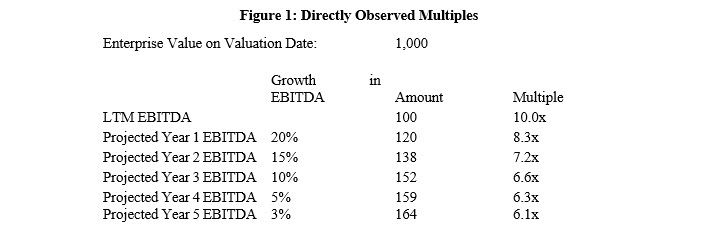
Multiples as of the terminal value date cannot be directly observed. We can directly compute multiples as of the valuation date by dividing a company’s enterprise value as of the valuation date by trailing and projected financial parameters as of the valuation date. However, we cannot directly compute multiples as of the terminal value date because we cannot observe stock and bond prices as of the terminal value date, which is several years after the valuation date.

See Figure 1 for a hypothetical example of multiples that can be directly observed on the valuation date. Observe that the EBITDA multiples decline each year. The decline in EBITDA multiples occurs because the numerator (enterprise value) remains constant while the denominator (EBITDA) increases each year.

Can Multiples as of the Terminal Value Date be Indirectly Observed?

Multiples as of the terminal value date cannot easily be indirectly observed either.

One may believe we can indirectly compute multiples as of the terminal value date through increasing the numerator to reflect the expected enterprise value on the terminal value date, as of the valuation date. The enterprise value is increased each year by assuming the business earns a rate of return equal to its weighted average cost of capital (WACC).

See Figure 2 for a hypothetical example of multiples that can be indirectly observed on the valuation date. Note that the EBITDA multiples decline at a slower rate in the earlier years (relative to Figure 1) and increase in the later years. The pattern for EBITDA multiples changes relative to Figure 1 because the numerator is no longer held constant. The EBITDA multiple decreases year-over-year when annual EBITDA growth is greater than the WACC. Conversely, the EBITDA multiple increases year-over-year when annual EBITDA growth is less than the WACC.

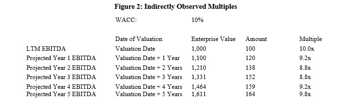
However, there is a flaw in the analysis contained in Figure 2: it assumes all the enterprise value is attributable to EBITDA projected to occur after the date of valuation. This is a faulty assumption for the terminal value because a (sizable) portion of the valuation as of the terminal value date is due to EBITDA (and ultimately cash flow) that is expected to occur between (a) the valuation date and (b) the terminal value date. Said differently, part of the reason why the enterprise value increased between the valuation date and terminal value date is due to free cash flow produced during that period.

The enterprise value as of the terminal date must be reduced to reflect the value, as of the terminal value date, of the free cash flow that is expected to be generated between the valuation date and terminal value date. This requirement, along with the need to arrive at an estimated WACC, adds a lot of subjectivity to the process and complicates an approach (use of exit multiples) whose main attraction is its perceived simplicity.

Triangulation with an Example that Uses Gordon Growth

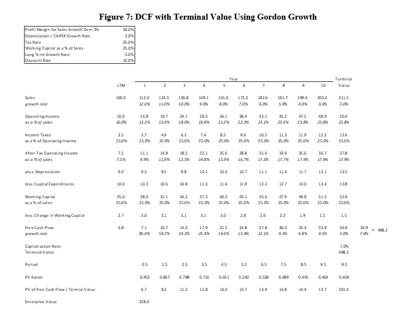
Let’s consider a business that is expected to have sizable growth for a few years before reaching a steady-state. See Figure 3 for the valuation of a hypothetical business that has four years of above steady-state growth. The terminal value is based on the Gordon Growth method after the business reaches a steady-state.

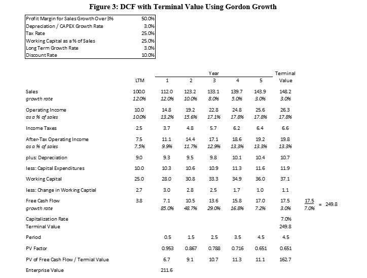
Let’s further assume that the valuation in Figure 3 is ‘correct.’ As shown in Figure 4, a 7.3x exit multiple (applied to projected year five EBITDA) is required to arrive at the same valuation in Figure 3.

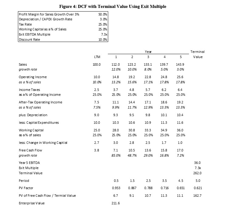
One nuance to keep in mind: the terminal value based on the Gordon Growth method is discounted back by 4.5 years whereas the terminal value based on the exit multiple is discounted back by five years. Both valuations identify the value of the business at the end of Year Five. The terminal value based on the Gordon Growth method is discounted back by 4.5 years because the Gordon Growth method assumes cash flows occur at the end-of-the-year, whereas this valuation assumes cash flows occur during the middle of the year.[1] 

Now let’s compare the multiples that are used or implied in this valuation. As shown in Figure 5, the one- year trailing EBITDA multiple applied for the terminal value (7.3x) is about the same as the two-year forward EBITDA multiple implied by the entire valuation as of the valuation date (7.4x). Assuming a guideline company existed that had the same profile as this company, the two-year forward multiple as of the valuation date is the appropriate proxy to use when determining the appropriate exit multiple as of the valuation date.

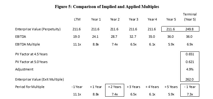
The comparison in Figure 5 highlights a key problem with exit multiples: it is not clear which time period of multiples should be used. Forward-looking multiples for values as of the valuation date tend to decrease as they look further out into the future because the numerator (enterprise value) remains constant while the denominator (EBITDA) is projected to increase. However, the terminal value typically uses a larger numerator because it is based on the company’s ability to create value at the end of the discrete projection period, not the beginning of the discrete projection period, and enterprise value is typically expected to increase during the interim period. These two issues move in opposite directions and it is not immediately clear why, in this example, the best proxy for the one-year trailing multiple as of the terminal value date is the two-year forward multiple as of the valuation date.

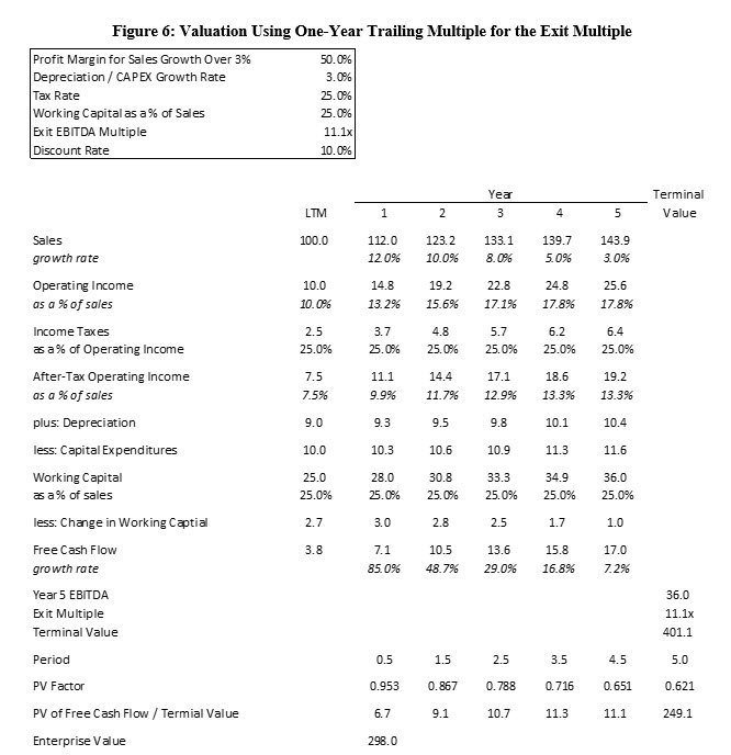
What would happen if this business was valued using the one-year trailing EBITDA multiple as of the valuation date? This could happen if the practitioner argues a one-year trailing multiple as of the valuation date is on an ‘apples-to-apples’ basis with the need to identify a one-year trailing multiple at the end of the discrete projection period. The enterprise value would be $298 million, as shown in Figure 6. Use of this multiple results in an overstatement of value of over 40%. This overstatement in value occurs because the expected growth outlook as of the terminal value date is much weaker than the expected growth outlook as of the valuation date.

More Growth = Greater Potential for Problems

Now let’s consider a company with  more growth before it reaches a steady-state. See Figure 7 for such a business.

Like the previous example, let’s further assume that the valuation in Figure 7 is ‘correct.’ As shown in Figure 8, an 8.6x exit multiple (applied to projected year 10 EBITDA) is required to arrive at the same valuation in Figure 7.

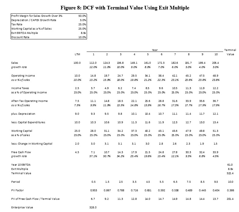
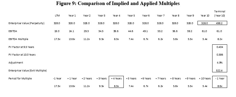
Now let’s compare the multiples that are used or implied in this valuation. As shown in Figure 9, the one- year trailing EBITDA multiple applied for the terminal value (8.6x) is about the same as the four-year forward EBITDA multiple implied by the entire valuation as of the valuation date (8.3x). Assuming a guideline company existed that had the same profile as this company, the four-year forward multiple as of the valuation date is the appropriate proxy to use when determining the appropriate exit multiple as of the valuation date. The proxy increased from two-year forward multiple to a four-year forward multiple because there is more growth in this scenario.

What would happen if this business was valued using the one-year trailing EBITDA multiple as of the valuation date? The enterprise value would be $533 million, as shown in Figure 10. Use of this multiple results in an overstatement of value of over 60%. This overstatement in value occurs because the expected growth outlook as of the terminal value date was much weaker than the expected growth outlook as of the valuation date.

Differences in Discount Rates

The examples in this article use a 10% discount rate. Some valuations may use significantly higher discount rates.

A significantly higher discount rate mitigates the effect to a degree but does not change the general observations. For example, the five-year valuation shown in Figures 3 and 4 still have the one-year trailing exit multiple (3.1x) roughly equal to the two-year forward multiple for the entire company as of the valuation date (2.9x) when a  20% discount rate is used. The 20% discount rate has a larger effect on the 10-year valuation shown in Figures 3 and 4 as the one-year trailing exit multiple (3.7x) is the mid-point between the forward two-year (4.0x) and three-year (3.4x) forward multiples for the entire company as of the valuation date.

Conclusion

It is very difficult to reliably identify the appropriate exit multiple for companies that are projected to have substantial growth during the discrete projection period. Practitioners should identify the implied long-term growth rate when using the Gordon Growth method as a sanity check to minimize the risk that they are using exit multiples that generate nonsensical results.

---

Michael Vitti,
CFA, joined Duff & Phelps in 2005. Mr. Vitti is a Managing Director in the
Morristown, NJ office and is a member of 
of the Dispute Consulting business unit. He focuses on issues related to
valuation and solvency. This article represents the views of the author and is
not the official position of Duff & Phelps, LLC.

Mr. Vitti can be contacted
at (973) 775-8250 or by e-mail to michael.vitti@duffandphelps.com.

[1] See https://quickreadbuzz.com/2018/07/18/the-discount-period-for-the-terminal-value/ for a more detailed discussion on this topic.