Terminal Values in DCFs

And Runaway Valuations

In a discounted cash flow analysis, a large portion of a firm’s value is typically attributed to the terminal value, i.e., the value beyond the projection period. Valuation presentations often show or discuss what happens to the firm’s value if the perpetuity growth rate (PGR) is changed. In this sensitivity analysis, it is common to see wild swings in valuations because the terminal value changes a lot when one changes the PGR for a given level of weighted average cost of capital (WACC). However, this large variation in terminal values could be a result of not linking the PGR and the amount of investment required during the terminal period to sustain the PGR.

In a discounted cash flow (DCF) analysis, a large portion of a firm’s value is typically attributed to the terminal value, i.e., the value beyond the projection period. Valuation presentations often show or discuss what happens to the firm’s value if the perpetuity growth rate (PGR) is changed. In this sensitivity analysis, it is common to see wild swings in valuations because the terminal value changes a lot when one changes the PGR for a given level of weighted average cost of capital (WACC). However, as I explain below, this large variation in terminal values could be a result of not linking the PGR and the amount of investment required during the terminal period to sustain the PGR.

The fundamental approach to estimating terminal values (TV) is typically calculated using the following formula:

[1] TV = FCF / (WACC – PGR) = (NOPAT – Net Investment) / (WACC – PGR),

where FCF is the expected free cash flow during the first year of the terminal period and is equal to net operating profit after tax (NOPAT) less net investment (i.e., capital expenditures plus increases in working capital minus depreciation and amortization). Although there are variations to this formula and how the inputs are calculated, for simplicity, we will use Eq. [1] and the definitions above to calculate the terminal value in the examples we discuss below.

To illustrate the issue at hand, let us consider the following example. Let us assume that during the first year of the terminal period, our subject firm has a NOPAT of $1,200, net investment of $200, PGR of two percent, and WACC of 12%. Using these inputs in Eq. [1], we know that the terminal value of the firm as of the end of the projection period is equal to $10,000. That amount is in the center of Table 1.

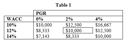
Now, let us assume that we want to know what would happen to the terminal value if we instead used a PGR of zero percent or four percent but keeping the WACC at 12%. As Table 1 shows, making these changes to the PGR results in a terminal value of $8,333 and $12,500, respectively. In this example, a PGR of four percent results in a terminal value that is 50% higher than the terminal value resulting from a PGR of zero percent. Thus, it appears that the choice of PGR has a dramatic impact on the valuation.

How large of an impact the change in PGR has on the terminal value also depends on the WACC used. As Table 1 shows, assuming a WACC of 10% and a PGR of zero percent results in a terminal value of $10,000, while assuming a WACC of 10% and a PGR of four percent results in a terminal value that is two-thirds higher at $16,667. On the other hand, assuming a WACC of 14% and a PGR of zero percent results in a terminal value of $7,143, while assuming a WACC of 14% and a PGR of four percent results in a terminal value that is 40% higher at $10,000.

The large swings in terminal value in the above illustration is due to the creation (destruction) of value when we move to a higher (lower) PGR by assuming the same level of net investment regardless of how fast (slow) the firm grows. To see why, we assumed in our illustration that a two percent PGR requires a net investment of $200. However, even when we doubled our PGR to four percent, we still invested only $200. This basically results in creating value out of no investment (i.e., a free lunch). This cannot be the case. On the other hand, when we cut the PGR to zero percent, we assumed to continue investing $200. That is, we invested too much and would not expect any positive return for a portion of the amount invested.

However, instead of a level investment amount regardless of the growth rate, it would be more reasonable to expect making larger (smaller) investments if one expected the firm to grow faster (slower). Thus, there should be a link between how much we invest and how much the firm would grow. Accordingly, a solution to the above problem is to link the net investment during the terminal period and the PGR. One way to do this is to use the following formula for the sustainable growth rate (i.e., the growth rate the company can sustain into perpetuity if all new investments come from the firm’s earnings):

[2] PGR = RONIC x Plowback Ratio = RONIC x (Net Investment / NOPAT),

where RONIC is the return on new invested capital.

If we know NOPAT and RONIC, we can then solve for the net investment that is required to achieve a given level of PGR. The NOPAT during the first year of the terminal period would usually be forecasted. As for the RONIC, two plausible choices for reasonable bookends in typical cases would be the following. First, under the assumption that into perpetuity and in competitive markets all excess returns are competed away, then we can assume that RONIC equals WACC. This means that all new investments would earn the WACC and, over time, the return on total capital (i.e., existing plus new capital) would converge to WACC. Second, under the assumption that the firm has some competitive advantage that it can sustain over the long run, then we can assume that RONIC equals WACC plus some excess return. However, competitive factors also limit the amount of excess return into perpetuity. Professor Damodaran suggests in his text that this excess return should be, at most, five percent. For our purposes, we will assume that WACC plus five percent is the maximum RONIC. In some cases, one of these assumptions could be more appropriate, while in other cases the more appropriate answer would be somewhere in between. Deciding what the appropriate RONIC is depends on the facts and circumstances of the valuation exercise, but for our current purpose we can illustrate how linking the net investment and PGR using these two RONIC assumptions affects our terminal value calculation.  

We first discuss the case when RONIC equals WACC. Like our example above, assume a firm with a NOPAT of $1,200, WACC of 12%, RONIC of 12%, and PGR of two percent. Using Eq. [2], we find that a net investment of $200 would support a two percent PGR. This results in a terminal value of $10,000. Likewise, using the same inputs but a PGR of zero percent results in net investment of zero dollars and a terminal value of $10,000, while using the same inputs as above but a PGR of four percent results in net investment of $400 and a terminal value of $10,000. The calculations are shown in Table 2.

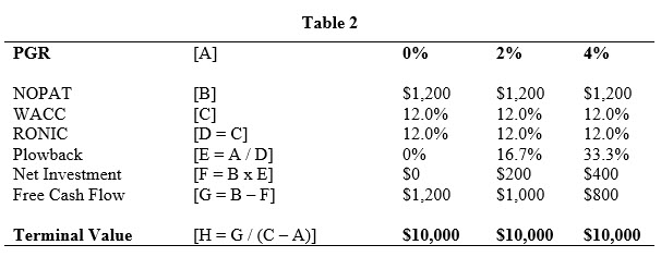
Note that the terminal value in Table 2, regardless of PGR, is $10,000. This is because when RONIC equals WACC, new investments do not earn excess returns (i.e., the NPV of those new investments is zero). Thus, we would expect that the terminal value when we assume RONIC equals WACC to be identical regardless of the PGR. This result is also confirmed by the calculations in Table 3 for different levels of WACC.

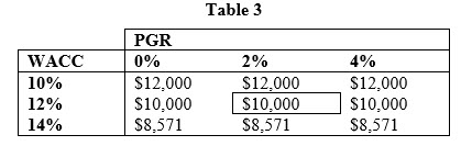
As Table 3 shows, when RONIC equals WACC, we should not expect any deviation in terminal values regardless of the PGR. Compared to Table 1, Table 3 shows higher terminal values in the case of a zero percent PGR, which is a result of not investing excessively when we expect slower growth. The increase in free cash flow given the lower net investment offsets the reduction in PGR. On the other hand, Table 3 shows lower terminal values in the case of a four percent PGR, which is a result of investing more when we expect faster growth. The decrease in free cash flow given the higher net investment offsets the increase in PGR.

Now, let us turn to the case of RONIC equals WACC plus five percent excess return. Like our example above, assume a firm with a NOPAT of $1,200, WACC of 12%, RONIC of 17%, and PGR of two percent. Using Eq. [2], we find the net investment of $141 would support a two percent PGR. This results in a terminal value of $10,588. Likewise, using the same inputs but a PGR of zero percent results in net investment of zero dollars and a terminal value of $10,000, while using the same inputs as above but a PGR of four percent results in net investment of $282 and a terminal value of $11,471. These calculations are shown in Table 4.

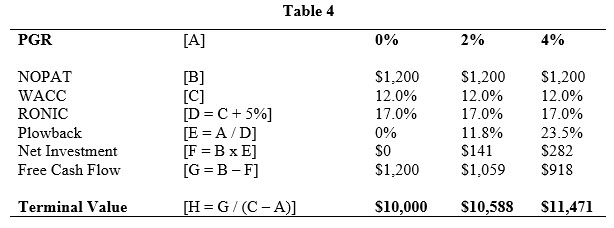
Compared to the assumption of RONIC equals WACC, the higher RONIC in this case (i.e., WACC plus five percent) results in a lower required net investment and, consequently, higher free cash flows. Thus, we would expect, all else equal, the terminal values in Table 5 would be higher than terminal values in Table 3 for any PGR greater than zero, which is what we observe.

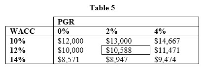
Although Table 5 still shows a deviation when one moves from a PGR of zero percent to four percent for a given level of WACC, the percentage deviation is much less than what is shown when the net investment is not linked to the PGR (i.e., Table 1). Specifically, the deviation for the WACC of 10% drops from 66.7% in Table 1 to 22.2% in Table 5, the deviation for the WACC of 12% drops from 50% in Table 1 to 14.7% in Table 5, and the deviation for the WACC of 14% drops from 40% in Table 1 to 10.5% in Table 5.

In summary, the effect of changing the PGR should not cause extremely large swings in the terminal value. These large swings could be prevented by linking the PGR to the net investment during the terminal period. The idea is that one should invest more if growth is expected to be faster and one should invest less if growth is expected to be slower. These offsetting factors would decrease or increase the terminal period free cash flows, respectively, and prevent runaway terminal valuations from occurring.

Opinions expressed herein are solely those of the author and do not reflect the views and opinions of Compass Lexecon or its other employees.

---

Clifford S. Ang, CFA, is a Senior Vice President at the Oakland, CA and Chicago, IL offices of Compass Lexecon. He is the author of Analyzing Financial Data and Implementing Financial Models Using R.

Mr. Ang can be contacted at (510) 285-1285 or by e-mail to cang@compasslexecon.com.