
R Programming and Ivy League Classes—For Free
There are a host of excellent statistical and optimization software packages available to valuation analysts and litigation support consultants. They are good, but also expensive. “R” is a programming language and software environment for statistical computing and graphics. The R language is widely used among statisticians and data miners for developing statistical software and data analysis. In this article, Lorenzo Carver introduces us to R and shows us how it can be integrated into one’s practice.
 A number of valuators make their first Application Program Interface (API) calls ever simply by copying and pasting a URL into a browser! Way to go! But we can go further towards our goal of each of you building your own industry risk premium (IRP) on-demand and free of charge.
We will rely on free price history data supplied by the Yahoo! Finance API employing the most widely used statistical computing language in the world know as “R” to programmatically access price history and convert it into to something that looks a lot like Beta.
I spoke about R and did a brief demo during one of my presentations at the National Association of Certified Valuators and Analysts (NACVA) 2015 Annual Consultant’s Conference in New Orleans. I was a little surprised to learn how few valuators were using it but very encouraged by the enthusiasm of the many people that came up to me afterwards to learn more.
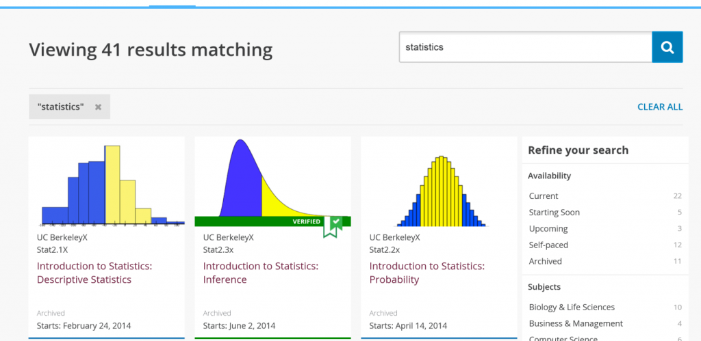
During that same presentation, and the subsequent “Conversations with the Masters–Panel Discussion and Q&A”, I mentioned a resource whereby world-class courses from Harvard, Columbia, MIT, Berkeley, and top universities around the world were available for free. That is not a typo—absolutely free of charge. EdX.org has free courses on statistics, machine learning (what used to be called statistical learning, in my opinion), programming, and not surprisingly, R programming.
Free Valuation Resources Links
Download R
Download Quantmod Package For R
Register For Free Classes at: edX.org
Yahoo! Finance API
Github
Bitbucket (Altlasian)

I brought this resource up as part of my suggestion that valuation practitioners brush up on statistics and apply regression analysis more efficiently using R. Coincidentally, one of the byproducts of using these two free tools (edX.org and R) is you can create even more resources that will be free for you to use as long as you practice valuation. So with that in mind, let’s jump right into to this installment of free valuation resources.
What is “R”?
Here is the description from the R-Project.org site: (A site I truly hope you visit; if you do not have the time, please encourage an analyst or associate to do so.)
“R is a free software environment for statistical computing and graphics. It compiles and runs on a wide variety of UNIX platforms, Windows, and MacOS. To download R, please choose your preferred CRAN mirror.”
The key words in the above description are: free, statistic, graphics, and runs. These words should convey the basic idea: it is free software that runs on pretty much any operating system a valuator is going to be using for production and that it performs statistical computations. If you know anything at all about R, you realize that description is quite an understatement. Wikipedia’s description of R is a little more compelling to those just being introduced to this amazing resource, I believe:
“R is a programming language and software environment for statistical computing and graphics. The R language is widely used among statisticians and data miners for developing statistical software and data analysis. Polls, surveys of data miners, and studies of scholarly literature databases show that R’s popularity has increased substantially in recent years.”
How Can “R” Benefit You as a Valuation Professional?
Valuation professionals, as well as credential granting organizations, often speak of “credibility.” A lot of times this is in the context of how opinions are developed, and supported in the context of a valuation report. That perspective is indeed important. But in the end, even the greatest wordsmith in the world has to yield to the power of science and basic math. R allows you to apply both to your valuations cost effectively, repeatedly, and at scale. If that does not get you excited, you honestly should not read any further.
How Hard is it to Learn “R”?
This is an important question. Like anything, there is a learning curve involved. In a world where we can point, click, and speak to machines that interpret our wishes instantly, the primary interface for R may seem like a throwback to many valuators. PLEASE do not be intimidated by the console, or command line interface. Just think of it as a word processor that interprets your commands into thousands of calculations and graphs, but is a bit particular about how you speak to it.
Now I am sure when I put it that way, half the audience is thinking “ok, this thing is hard to use and learn.” But if you are doing anything complex in Excel today, advanced Visual Basic for Application scripts, sophisticated macros, or solver templates, here is the reality: R is easier, more auditable, and more replicable. Don’t believe me? We are going to prove it as part of building your own IRP.
Easier Than Excel?
In my business, we typically test things with users over and over again before we take them to market in order to get an idea of how hard they are to digest; therefore if it is worth pursuing a product before we refine the interface. I take a similar approach with our valuation services and with these articles.
I tested a version of this article that tried to walk moderate users of Excel through how to automatically calculate Beta in Excel, pulling pricing data for the subject companies automatically, pulling data for the index automatically, placing that in the appropriate cells, calculating periodic returns, and running a regression analysis, slope, or covariance calculation to get an indication of beta. That run-on sentence is deliberate to give you a feel for the steps.
The first run through of the description took 20 pages to effectively describe and about as many hours for someone knowledgeable about valuation and Excel, but with no programming experience, to convert into a usable routine. While that is not bad for someone truly motivated, it is a failure if the goal is to get people excited about using programming (cut, paste, attach style—CPA) to improve their valuations.
After you have installed R on your laptop or desktop, you will do all of this in a matter of minutes simply by running less than 10 lines of code in R that I wrote for you. Moreover, you can (and should) edit that code to make it your own.
Installing “R”
To get started, install R on your machine. Typically you would go to the R-Project.org site and navigate to “mirror” site that has the installation files. But since that ads a little of time to the process, I have provided a deep link to the installation file from the Berkeley (UC Berkeley) mirror site.
This deep link works for Windows installations:
http://cran.cnr.berkeley.edu/bin/windows/base/R-3.2.1-win.exe

This link works for Mac (Mavericks and later) installations:
http://cran.cnr.berkeley.edu/bin/macosx/R-3.2.1.pkg
After you have downloaded the installation files, double click, ignore the Windows warnings, and accept all default installation settings. That is it! You have installed one of the most widely used statistical packages on your machine free of charge.
I run R on multiple machines and on multiple operating systems. The main machine I travel with has both Windows 8 (which runs the primary valuation software my client’s license from us) and MAC OS X (which runs the tools I use to develop iOS apps).
I am not an expert in R, but can tell you my experience has been that things simply do not always work exactly the same way in the Mac version as the Windows version. But it will probably take you a long time of playing with R before you encounter these differences. Some of these differences appear to relate to packages, but none of these differences should make a difference for the exercise (script) you will be running today.
Quantmod: The Power of “R” Package
One of the most powerful benefits of R is “Packages” and if you are doing anything that involves grabbing financial data (especially free financial data), Quantmod is the first package not included with the base R installation that you will want to install. We will get into more detail on what packages really are in later installments of Free Valuation Resources, but if you have ever played a video game, opted for an upgraded engine, or seen a superhero movie hopefully these analogies will paint a mental picture of what the right R Package can do for you.
I like to describe what R Packages do for R users as similar to what “Power-Ups” do to video game users: they allow you to go further faster, rack up bonus points, and ideally, make it to the next level. You could say they give your base installation of R superhero powers. To use those powers, all you have to do, in many cases, is download and install the package, using the “install.package“ function in R. In the case of this example, you do not even have to do that, since I have included the install.packages(quantmod) command in the script file you will run after installing R.
Quantmod was developed by Jeffrey A. Ryan. It is available under the GNU General Public License, which means it is “free”, according to the Free Software Foundation’s license language “…intended to guarantee your freedom to share and change all version of a program—to make sure it remains free software for all its users.”
Ever wanted to build your own equity risk premium from scratch? Quantmod is probably the easiest way to do so, requiring just a few lines of codes (which you can copy and paste into R) to pull pricing history from free API’s such as Yahoo! Finance and pull risk free rates from the St. Luis Fed’s FRED API.
More specific to your objective of enabling you to build your own industry risk premium from scratch, you can calculate beta’s for any security from scratch with as few as seven lines of code, even less if you install other packages before loading the script below. Don’t believe me? Give it a try.
Getting an Indication of Beta From Scratch—For Free
Before we paste the code below, let’s recall why we might want to use beta as a means of arriving at an IRP. The obvious reason would be because that is one of the key steps used by Ibbotson when arriving at their IRP published in the traditional Stocks Bills Bonds and Inflation (SBBI) Valuation Yearbook. There are a number of caveats to how SBBI weights various companies based on line of business and how they have changed the approach over time, but for now we should just agree that calculating beta is part of the process for arriving at an IRP using their methodology.
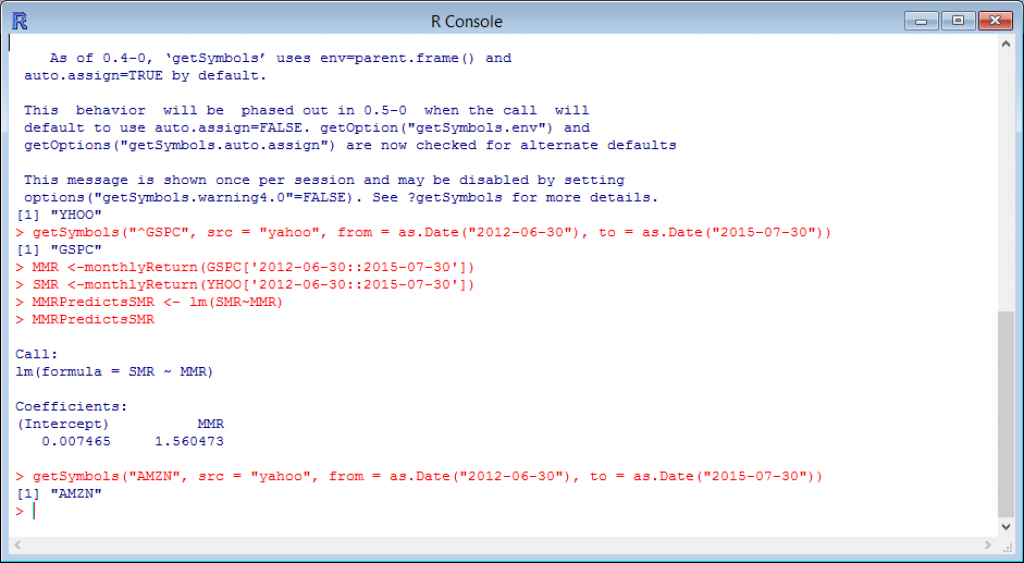
So to calculate one indication of beta, using an assumption for periodicity (end of month, three years of pricing history) consistent with the beta published by Yahoo!, simply open R after you have installed it and paste the following seven lines into the R console:
library(quantmod)
getSymbols(“YHOO”, src = “yahoo”, from = as.Date(“2012-06-30”), to = as.Date(“2015-07-30”))
getSymbols(“^GSPC”, src = “yahoo”, from = as.Date(“2012-06-30”), to = as.Date(“2015-07-30”))
MMR <-monthlyReturn(GSPC[‘2012-06-30::2015-07-30’])
SMR <-monthlyReturn(YHOO[‘2012-06-30::2015-07-30’])
MMRPredictsSMR <- lm(SMR~MMR)
MMRPredictsSMR
You will be returned the following by R:
Coefficients:
(Intercept) MMR
0.007465 1.560473
The slope, 1.56, is one indication of the beta for this particular stock.
Now, go to Yahoo! Finance and enter the symbol YHOO. Look at the Beta, provided by a service as opposed to calculated live, and you will see that your calculation in R is very close.
You will note that it works here easily because we deliberately picked a stock with no dividends or splits. Now, try it on your own with another tech stock that does not pay dividends and has not had a stock split for the past three years (such as Amazon—AMZN).
In this case, there is no code for you to simply CPA (copy, paste, attach), but there is also very few keystrokes required to calculate the beta from scratch. You will just use your keyboards’ up and down arrow keys to edit some of the code you pasted previously. As you do it, I will walk you through what the variables are and how they were used to get an indication of beta.
Step 1: With your cursor active in the “R Console”, click your up arrow key once.
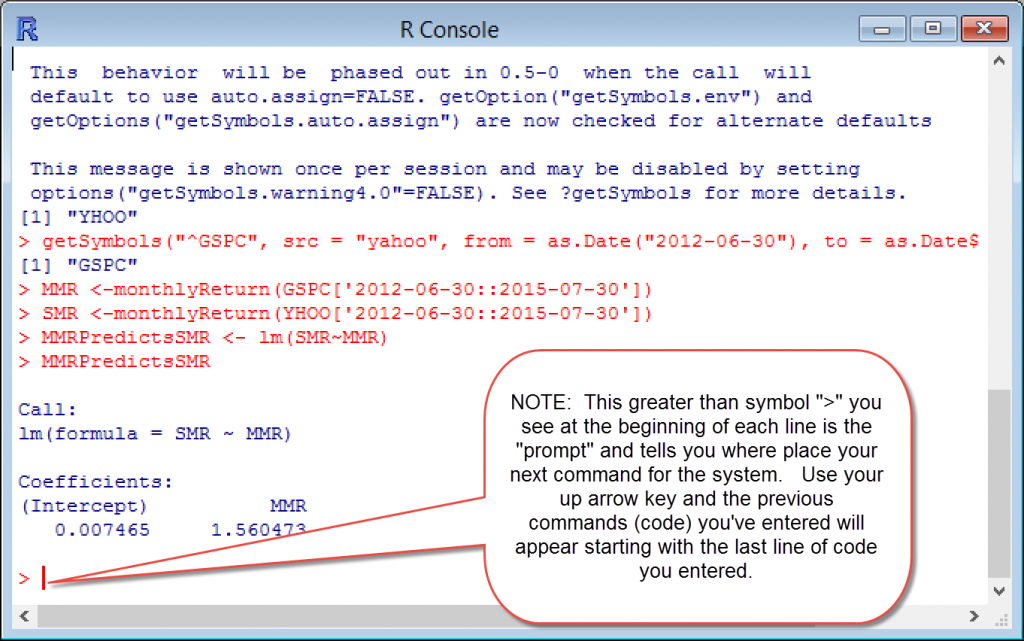
You will see the most recent (last) line of code entered appear at the command line, as shown in the illustration below.
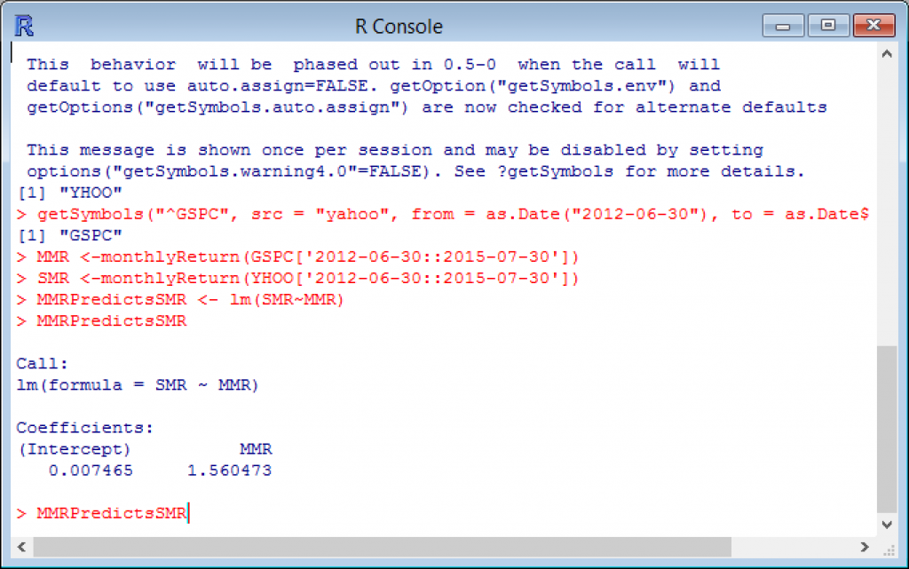
However, we do not need this line of code just yet. Instead, keep clicking your up arrow until you see the “getSymbols(“YHOO”,…” line displayed at the prompt, as shown in the image below.
Step 2: Simply use your left arrow key to go back on the line until you get to the characters “YHOO” on that line and replace them with the ticker “AMZN”, another tech company with no dividends and no stock splits to screw up our simplified example of building your own indication of beta from scratch.

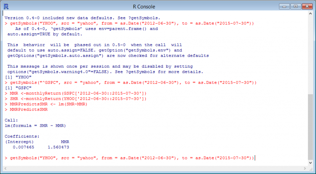
After you have replaced “YHOO” with “AMZN” just hit your keyboard’s return (Enter) key and R will return this: [1]
Congratulations!
You just brought three years of complete stock price history for Amazon by editing four characters. However, in order to match the third-party published beta calculation we need to calculate beta using the same number of periods and with the same assumptions. In our case, that means we want three years of monthly returns. I created a “variable” named Subject Monthly Returns (SMR) to hold the value of these monthly returns for the subject company.
Step 3: With your cursor active in the “R Console”, click your up arrow again until you get to the line where I assign values to the SMR variable.
Without knowing anything about R or Quantmod, you can probably deduce that the variable SMR currently holds pricing data for Yahoo! ticker “YHOO.” But we now want to calculate a beta indication for Amazon, ticker “AMZN” so the easiest way to do that is to simply replace the stock price history data (value) currently held in my variable named SMR with Amazon stock price history for the same period.
Warning: Do not confuse “src=yahoo” with the ticker “YHOO.” “src” is just telling Quantmod what data provider to request the price history from (the Yahoo! Finance API is the source of pricing data in this case). 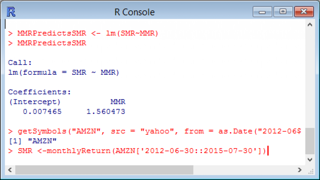
As in the previous line you edited, use you left arrow key to go back on the line until you get to the characters “YHOO” on that line and replace them with the ticker “AMZN.”
After you have replaced “YHOO” with “AMZN” just hit your keyboard’s return (Enter) key. You will simply be presented with the R prompt (>). If you would like to see what was created for you by the Quantmod package, just type SMR (the variable you assigned Amazon monthly returns to) and R will print the following to the console:
> SMR
monthly.returns
2012-07-31 0.017444396
2012-08-31 0.064166313
2012-09-28 0.024368643
2012-10-31 -0.084263949
2012-11-30 0.082270617
2012-12-31 -0.004681642
2013-01-31 0.058317078
2013-02-28 -0.004632810
2013-03-28 0.008400504
2013-04-30 -0.047581495
2013-05-31 0.060635964
2013-06-28 0.031537851
2013-07-31 0.084734772
2013-08-30 -0.067193380
2013-09-30 0.112677069
2013-10-31 0.164374301
2013-11-29 0.081284499
2013-12-31 0.013134531
2014-01-31 -0.100554192
2014-02-28 0.009506828
2014-03-31 -0.071057748
2014-04-30 -0.095846807
2014-05-30 0.027685473
2014-06-30 0.039129776
2014-07-31 -0.036301524
2014-08-29 0.083229560
2014-09-30 -0.048961794
2014-10-31 -0.052660994
2014-11-28 0.108623142
2014-12-31 -0.083540065
2015-01-30 0.142355380
2015-02-27 0.072292909
2015-03-31 -0.021201594
2015-04-30 0.133512476
2015-05-29 0.017663265
2015-06-30 0.011322566
2015-07-30 0.236517807
Step 4: With your cursor active in the “R Console”, click your up arrow again until you get to the line where we fit the linear model (lm) and assign its value to the variable I named Market Monthly Returns Predicts Subject Monthly Returns (MMRPredictsSMR).
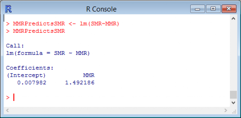
As in the previous example, you can check your homemade beta calculation by going to Yahoo! Finance and entering the symbol AMZN and seeing if it is close to the 1.49 that should print out to your screen as illustrated above.
NOTE: Although we have not dug into details (since for now this is a copy and pasting exercise primarily just to give you confidence in how easy it is to do powerful analysis in R with little or no programming skills). However, like everything, you need to understand the syntax in order to get results in the real world.
The syntax for R’s lm() function that we used to run a single linear regression was simply a response (or dependent variable) followed by the tilde symbol (~) and finally followed by the predictor (or independent variable). The order matters, but we will cover more on that in a future installation. For now, you should feel really good about:
- Pulling in years of daily pricing data for two subject companies;
- Pulling in years of daily pricing data for an index (benchmark) representing the market;
- Converting that pricing data into periodic returns;
- Storing each of these items above in containers that can be reused, edited, and shared to insured consistent and replicable results; and
- Running a regression model you built that gives you an indication of beta free of charge simply by copying and pasting a few characters.
Have questions? Feel free to send me a note on LinkedIn: https://www.linkedin.com/in/lorenzocarver
[divide]
Lorenzo Carver, MS, MBA, CVA, ABV, CPA is Founder and CEO of Liquid Scenarios, an automated valuation software, data, and services company responsible for the first one click valuation solution for complex, illiquid securities. He is the inventor of the Carver Import Algorithm, Search2Model, a patented valuation technology and author of Venture Capital Valuation published by John Wiley & Sons. Mr. Carver has over 40,000 hours of valuation related experience and his Liquid Scenarios automated valuation software, services and data is used to value thousands of venture backed companies, including industry changing successes like Facebook, Twitter, Dropbox and Uber. Mr. Carver can be reached at: (650) 690-2169 or e-mail to: bpcentral@gmail.com.