
Basic Statistics
A good start for a forensic accounting engagement
Statistical data is commonly presented in litigation reports. The data provides valuable information to test the hypothesis. This article provides an introduction of how some statistical techniques that are readily available can be used in practice.
 For some litigation support professionals, the term statistics often invokes the image of a highly technical number cruncher that was the mathematical genius in college. Yet, there are some basic statistical concepts that are easy to do. The application of these concepts provides a wealth of information about a set of data, such as financial statement information, invoices, purchase orders, and other accounting information subjected to investigative scrutiny in a forensic accounting engagement. Of greater importance is the role statistical analysis plays in detecting unusual variations in the data set under review. This article focuses on the use of Z-Score calculations and the role they play in determining anomalies in financial information.
The official formula for calculating a Z-score is the observation number minus the mean divided by the standard deviation or (X – mean)/standard deviation) of the population. In order to calculate Z-scores, one must first do the preliminary calculations of the mean and the population standard deviation, but these are very easy to calculate using Excel formulas. The mean is quite simple—it is the average of the population using = average (n1, n2, n3,) in the statistical formulas in Excel, or better yet, in Excel 2007 and later versions, scrolling down a column for totals, the average of the column is also available to view.
The standard deviation of the population is just as easy using the Excel formula =STDEV.P (n1, n2, n3, etc.). The data analysis tools provided in Excel as an add-in to the standard program will also calculate these by using the “descriptive statistics” tool and will provide other information concerning the population, such as the range, as well as the minimum and maximum amounts within the population. Once these are completed, Excel makes the calculation of the Z-score easy by using the “standardize” formula in Excel.
For example, if the observation number X is equal to $1,388,977, the population mean is $4,675,840, and the population standard deviation is $9,161,132; the Z-score calculation for the number X is -.36. Negative numbers are not relevant when analyzing calculations to the methods noted in the following paragraphs, but they do indicate placement above or below the standard deviation of the mean.
The first method used to analyze Z-scores is known as Chebyshev’s Theorem1. It states that at least 75 percent (rounded) of all observations fall within two standard deviations of the mean, at least 89 percent (rounded) of all observations fall within ± three standard deviations of the mean, and at least 94 percent (rounded) of all observations fall within ± four standard deviations of the mean. Chebyshev’s Theorem applies to a population of data points that do not have a bell-shaped curve known as a normal distribution or a symmetrical distribution. The other method used applies to a symmetrical distribution (the bell-shaped curve) known as the Empirical Rule2. With the Empirical Rule, approximately 68 percent of all observations fall within ± one standard deviation of the mean, approximately 95 percent of all observations fall within ± two standard deviations of the mean, and approximately 99.7 percent of all observations fall within ± three standard deviations of the mean.
In order to interpret the Z-score calculation, the user must decide which method is appropriate based on the “shape” of the data. One can easily determine the shape of the data by drawing a histogram or using the bar chart in Excel and adjusting the width between the bars. The following charts of financial data were made in Excel to determine shape of the population in order to determine which method would be appropriate to use in analyzing the Z-score calculations.
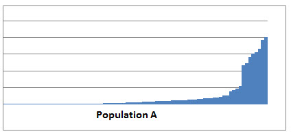
In the first chart, Population A, represents a population of financial data that is not symmetrical in nature since it does not have a classic bell-shape curve look to it. Any Z-score calculations made from this data would need to be analyzed using Chebyshev’s theorom to determine whether the data contained outliers within its population.
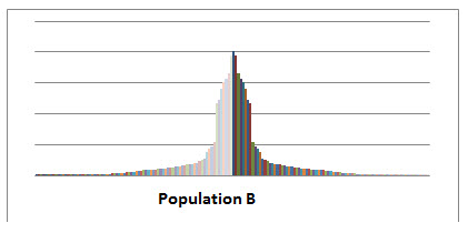
In the second chart, Population B, represents a population of financial data that is symmetrical in nature, and the Empirical Rule will apply to Z-score calculations for observation numbers within this population in order to determine if outliers exist within the population.
If the observation number is part of a non-symmetrical population, such as Population A, Chebyshev’s Theorem would apply. For example, a calculated Z-score of -.36 indicates that the observation number falls .36 standard deviations below one standard deviation of the mean and falls within two standard deviations of the mean indicating the observation number is not unusual since at least 75 percent of observations to fall within two standard deviations of the mean.
What happens when the Z-score is ±3.21 or ±4.14? The Z-score of ±3.21 falls within three standard deviations of the mean suggesting the possibility that this observation number may be unusual since 89 percent of observations fall more than three standard deviations of the mean. A Z-score in this range suggests the possibility of the observation number being an outlier to the population. A Z-score of ±4.14 falls more than four standard deviations from the mean suggesting this observation number is definitely an outlier. In other words, the farther the observation number is from the two standard deviations of the mean, the more likely the number is an outlier of the population.
When using Chebyshev’s Theorem, the important points to remember are:
- A Z-Score that is less than -3 or more than 3 is unusual and only occurs about 11 percent of the time. In such cases, it is possibly an outlier. Generally, additional study is required before determining the final verdict.
- A Z-score that is less than -4 or more than 4 occurs less than 6 percent of the time. This scenario is very unusual, and an outlier is probably involved.
Moving on to a population representative of Population B, if the observation number X is equal to $400,032, the population mean is calculated as $320,728, and the population standard deviation is calculated as $94,096. The Z- score calculation for the number X is .842 and falls within one standard deviation of the mean using the Empirical Rule. What happens when there is a Z-score calculation of ±2.89 under the Empirical Rule? The observation with this Z-score indicates that it falls within 95 percent of two standard deviations of the mean and possibly an outlier of the population. Of course, a Z-score of ±3.21 falls within three standard deviations of the mean and suggests the observation number is an outlier of the population.
In using the Empirical Rule, the important points to remember are:
- If a Z-Score is less than -2 or more than 2, it occurs only about 5 percent of the time, so it is unusual and possibly an outlier. Generally, a larger sample is required before determining the final verdict.
- If a Z-score is less than -3 or more than 3, it occurs less than 0.3 percent of the time, so it is very unusual and probably an outlier.
Since ABC Company was experiencing some unexplainable cash flow issues, management asked that an analysis of their financial information be performed in order to determine the causes of the cash flow problems so the company could resolve those issues. The owners were experiencing increased sales in their products with very little product returns or extreme delinquency in the collections of their receivables, yet the company was not able to keep the payments to their vendors current. In determining the approaches and various analyses to use, one of the first steps was to compile the trial balances for the past five years and the current year into one population to look for unusual variances. Z-scores were calculated on the various line items of the trial balances over a period of six years once the shape of the population had been determined.
The shape of the population of the financial information for ABC Company was similar to Population A shown above, so Chebyshev’s Theorem was used to analyze the Z-scores. In both the current year and the prior year, the Z-scores for sales were 3.08 and 2.88 respectively, but the Z- scores for the cost of raw materials were 4.23 and 4.03 respectively. In the other prior years under study, the Z-score calculations for both sales and raw materials were less than two standard deviations from the mean. Using the guidelines for Z-score calculations under Chebyshev’s Theorem, the amounts in the trial balances for raw materials indicated these numbers were probably outliers of the population. Using further analytical procedures and inspection of specific documents, the results of the analysis revealed embezzlement activities with those personal costs being posted in the raw material account.
By first calculating the Z-Scores, the calculations pointed to specific areas within the financial statements of ABC Company for further analysis and investigation. Effective? Yes, and more importantly, these calculations are simple to execute, easy to interpret, and point to outliers in a population that may be indicative of possible fraudulent activity.
Pam Mantone, CPA, CFF, CFE, FCPA, CITP, CGMA, MAFF, is a senior manager with Decosimo’s Chattanooga, Tennessee, office. She provides litigation support services with emphasis on forensic accounting and fraud examinations and also practices in areas of audit and attestation primarily serving not-for-profits, governments, and financial institutions. Pam can be reached at (423) 756-7100 or pammantone@decosimo.com.
1Pace, Larry A., “Statistical Analysis Using Excel 2007,” Pearson Education, Inc., 2011.
2Ibid.


