The Valuation Impact of Using the Wrong Leverage Ratio to Unlever Betas

Recognize and Avoid Substantial Valuation Differentials

One of the critical inputs in the capital asset pricing model (CAPM) is beta. In practice, there are two typical ways beta is estimated. Making an incorrect assumption could lead to substantial valuation differentials of over 10% in many cases and can lead to valuation differentials of over 50% in some instances. In addition, our analysis indicates that we would not be able to tell the direction and magnitude of the valuation differential in advance unless the correct calculation is performed.

One of the critical inputs in the capital asset pricing model (CAPM) is beta. In practice, there are two typical ways beta is estimated. First, we run a regression of the subject firm’s return on the market’s return and plug that beta directly into the CAPM.[1] Second, we rely on peer company betas.[2] In this approach, we identify peer companies, estimate the beta for each peer company, unlever the peer company beta using the current period leverage, take the average or median peer company beta, relever the average or median peer company beta using the subject firm’s target capital structure, and then plug this relevered beta into the CAPM formula. These approaches typically assume that the average regression period beta, whether it is for the subject firm in the first approach or each of the peer firms in the second approach, is equal to their current period leverage. However, this assumption is likely to be invalid because leverage ratios of firms often change over time.[3] As we show below, making this incorrect assumption could lead to substantial valuation differentials of over 10% in many cases, and can lead to valuation differentials of over 50% in some instances. In addition, our analysis indicates that we would not be able to tell the direction and magnitude of the valuation differential in advance unless the correct calculation is performed.

Before we delve into the details of the valuation implications, we first discuss the issue at a conceptual level. The process of unlevering betas is intended to remove the effects of leverage embedded in the beta. The regression beta reflects the average effect over the regression period. Consequently, the levered returns used to estimate the regression beta is based on the average leverage during the regression period. The preceding is not a novel concept, but is recognized in valuation textbooks.[4] Therefore, unless the average leverage ratio during the regression period is coincidentally identical to the current period leverage ratio, unlevering the regression beta using the current period leverage ratio does not properly remove the effects of leverage in the regression beta. Despite this, virtually all beta calculations we have encountered in practice ignore the use of the average regression period leverage.

Data and Methodology

We use the components of the S&P 400 Midcap Index as of December 31, 2019 as our sample, which give us a broad sample of firms.[5] In our analysis, we first estimate the regression beta for each firm using five years of monthly returns ending December 31, 2019. We use the S&P 500 Index as the market proxy in all regressions. We also estimate regression betas using two years of weekly returns ending on December 27, 2019, the last Friday in 2019. This is also a common estimation period and return frequency used in practice. For example, Yahoo Finance reports betas calculated using five years of monthly returns, while the default beta calculation on the Bloomberg terminal uses two years of weekly returns.

To calculate the base case valuation (i.e., our proxy for what is typically done in practice), we plug the regression beta directly into the CAPM to arrive at a cost of equity. We then use that cost of equity to value a $100 annuity.

Next, to calculate the alternative valuation, we unlever the beta using the Hamada formula and the average leverage ratio during the regression period.[6] We then relever the unlevered beta using the target leverage ratio, which we assume to be the current period leverage ratio. Finally, we plug this relevered beta into the CAPM to arrive at a cost of equity and use that cost of equity to value a $100 annuity.

To analyze the effect of using the improper leverage ratio for larger firms, we also perform the same analysis described above using the components of the Dow Jones Industrial Average.

Returns and firm-specific leverage data are obtained from Capital IQ. To calculate the CAPM cost of equity, we assume an equity risk premium of 6% and a risk-free rate of 2.25%.[7]

Valuation Differentials

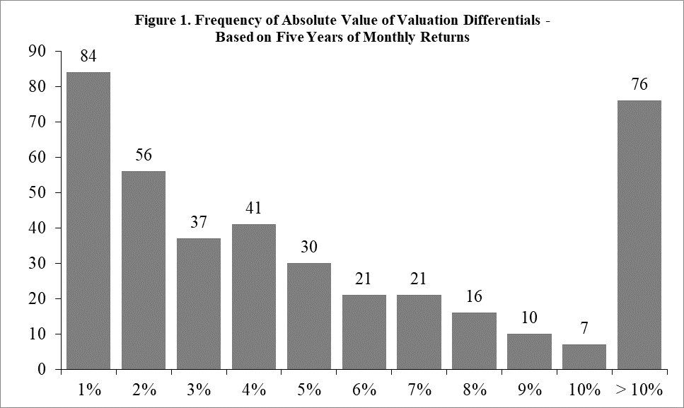
We now compare the base case valuation and the alternative valuation for each firm. In our analysis, we treat overvaluations (i.e., positive differentials) and undervaluations (i.e., negative differentials) the same. Thus, for each firm, we calculate the absolute value of the percentage difference of the two valuations. As Figure 1 shows, although 248 or 62% of the firms in our sample have valuation differentials of 5% or less, 76 or 19% of the firms have valuation differentials of over 10%. For most analysts, it would likely be concerning if there was a 19% chance of having a valuation error of at least 10%.

Moreover, we can also look at the details of some of the firms with the largest valuations to glean certain insights into the source of the valuation differential. Table 1 shows the 10 firms with the largest absolute valuation differentials. The largest valuation differential is for Chesapeake Energy Corp., which has a regression beta of 2.38. This yields a CAPM cost of equity using the regression beta of 17% and the value of the annuity is $605. Over the five-year regression period, the average debt-to-equity ratio for Chesapeake is 280% and average preferred-to-common equity ratio is 60%. Using these average leverage ratios, the unlevered beta for Chesapeake is 0.62. Assuming current period leverage ratio equals the target leverage ratio, the target debt-to-equity ratio is 587% and target preferred-to-common equity ratio is 102%. These leverage ratios are substantially higher than the average leverage ratios over the regression period. Using these target leverage ratios, the relevered beta is 4.15. This yields a CAPM cost of equity of 27% and the value of the annuity is $368. Thus, for Chesapeake, using the improper leverage ratios results in an overvaluation of 64%. Table 1 also shows that the use of the improper leverage ratio to unlever beta can lead to undervaluations (e.g., WW International, Inc. and Caesars Entertainment Corporation) when the target leverage ratios are lower than the average regression period leverage ratios.

The above analysis assumes a tax rate of 21%, so we can isolate the impact of the use of the improper leverage on the analysis. However, because the five-year estimation period includes three years (2015–2017) during which the marginal tax rate was 35% and two years (2018–2019) during which the marginal tax rate was 21%, the tax rate used when unlevering the betas in the alternative case should be 29.4%, which is the weighted-average tax rate during the regression period. The qualitative conclusions reported above do not change when using this weighted-average tax rate.

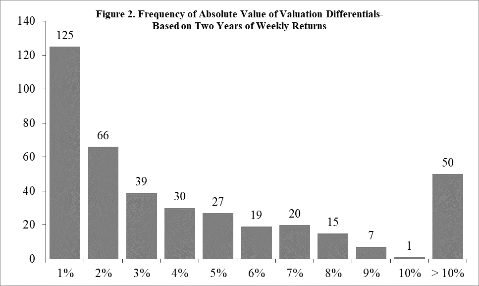
These effects are not isolated to regression betas estimated using five years of monthly returns. Figure 2 shows the absolute value of the percentage difference in valuations based on betas estimated using two years of weekly returns. As the chart shows, although there are 287 or 72% of the firms in our sample had a valuation differential of 5% or less, 50 or 13% of the firms have a valuation differential of over 10%. For most analysts, it would likely be concerning if there was a 13% chance of having a valuation error of at least 10%.

Looking more closely at the 10 largest valuation differentials, we can observe from Table 2 that there are also very large valuation differentials when using two years of weekly returns to estimate the regression beta. For example, Chesapeake Energy Corp. has a valuation differential of 48% and Meredith Corp. has a valuation differential of 31%. Table 2 also  shows that there are only four firms that overlap with Table 1. Moreover, even for the firms that overlap in both tables, we can see that the average leverage ratios are different. For example, Chesapeake Energy Corp. had an average debt-to-equity ratio of 333% over the most recent two-year period, while it had an average debt-to-equity ratio of 280% over the most recent five-year period. Similarly, Meredith Corp. had an average debt-to-equity ratio of 107% over the most recent two-year period, while it had an average debt-to-equity ratio of 63% over the most recent five-year period. The above indicates that different regression periods could lead to different magnitudes of the valuation differential. Therefore, we cannot assume that a firm that has a small valuation differential in one regression period will also have a small differential over a different regression period.

Finally, in unreported results, we also perform the same analysis as the above for the 30 firms in the Dow Jones Industrial Average. The components of the Dow are larger and more stable than the midcap firms we used in our earlier analysis. Despite this, we still found large valuation differentials. For example, J.P. Morgan has a 13% valuation differential using a five-year monthly regression beta and IBM has an 8% valuation differential using a two-year weekly regression beta.

Conclusion

The above analysis shows that using the improper leverage ratio to unlever betas can lead to substantial valuation differentials. In a significant percentage of cases, the valuation differentials can exceed 10%. In some cases, the valuation differentials can exceed 50%. The size of the error rate is likely concerning to most valuation analysts. We also show that the direction and magnitude of the valuation differential cannot be determined without performing the proper calculation, as the combined effect of the choice of estimation period and return frequency plus the difference in average and target leverage ratios cannot be known a priori.

Opinions expressed herein are solely those of the authors and do not reflect the views and opinions of Compass Lexecon or its other employees.

---

Clifford S. Ang, CFA, is a senior vice president in the Oakland, CA and Chicago, IL offices of Compass Lexecon. He is the author of Analyzing Financial Data and Implementing Financial Models Using R.

Mr. Ang can be contacted at (510) 285-1285 or by e-mail to cang@compasslexecon.com.

Andrew Lin, CFA, CAIA, is a vice president in the Chicago, IL office of Compass Lexecon.

Mr. Lin can be contacted at (312) 322-0204 or by e-mail to alin@compasslexecon.com.

 

[1] See, for example, S. Pratt, 2008, Valuing a Business, 5th ed., McGraw-Hill, at 187 (“One common method for calculating beta…[t]he computation may be performed by carrying out a regression of the excess stock returns against the excess market returns.”) & T. Koller, M. Goedhart, D. Wessells, 2015, Valuation, 6th ed., Wiley, at 283 (“Since beta cannot be observed directly, you must estimate its value. The most common regression used to estimate a company’s raw beta is the market model: In the market model, the stock’s return (R_i), not price, is regressed against the market’s return.”).

[2] See, for example, T. Koller, M. Goedhart, D. Wessels, 2015, Valuation, 6th ed., Wiley, at 282 (“To best implement the CAPM, for instance, we recommend using a peer group beta, rather than raw regression results.”).

[3] H. DeAngelo, R. Roll, 2015, “How Stable Are Corporate Capital Structures?,” The Journal of Finance 7, 373–418 (“Capital structure stability is the exception, not the rule, occurs primarily at low leverage, and is virtually always temporary, with many firms abandoning low leverage during the post-war boom.”).

[4] See, for example, A. Damodaran, 2018, The Dark Side of Valuation, 3^rd ed. (Pearson) at 42 (“The debt-to-equity ratio over the regression period is embedded in the beta.”).

[5] According to the S&P MidCap 400 Index Fact Sheet as of December 31, 2019, the index is comprised of 400 mid-sized companies in 11 different sectors with market capitalizations ranging from $1.1 billion to $12.6 billion with a median market capitalization of $4.3 billion as of December 31, 2019. However, Genesee & Wyoming Inc. was acquired on December 30, 2019 and was not replaced by RH until January 2, 2020. Hence, our total sample only includes 399 firms.

[6] To isolate the valuation differentials due to the use of improper leverage ratios, we assume debt betas for each firm equal zero. However, assuming a non-zero debt beta does not qualitatively alter our conclusion.

[7] The 6% ERP is based on the midpoint of the range of ERPs found in textbooks of 5% to 7%, while the risk-free rate is the yield on a 20-year Treasury security as of the end of 2019.