How to Test the Monte Carlo Model

Sanity Checks to Keep it Real and Defensible (Part II of II)

This is the second QuickRead article on interest rate volatility and modeling, read Part I here. As valuation professionals, we know that we need to develop and test the interest rate assumption. Valuation professionals also need to understand the impact that an interest rate used will have on the cash flows and value of the firm, and ensure that the rate is real and defensible. Monte Carlo modeling allows us to test the underlying assumptions. Time to put it all together.

This is the second QuickRead article on interest rate volatility and modeling. As valuation professionals know, we need to develop and test the interest rate assumption. Valuation professionals also need to understand the impact that the interest rate used will have on cash flows and the value of the firm, and ensure that the rate used is real and defensible. Monte Carlo modeling allows us to test the underlying assumptions. Time to put it all together.

This article will address valuation spreadsheets built on discounting future free cash flow. The techniques should scale to any level of granularity, any time horizon, and whether you assume a perpetuity in your last column.

You could select a range of values for the hurdle rate and other uncertain inputs. Then run the spreadsheet a few times, yielding perhaps best, worst, and most likely cases. Even if you do a great job, the results will not show the relative likelihood for each case, or the samples you did not pick. Also, my experience is that it is very hard to eyeball those interactions and dependencies.

I would argue instead for running a Monte Carlo simulation within your spreadsheet. No one makes this case better than Sam Savage of Chancification in his many articles and his book, “The Flaw of Averages.” Here are a couple of Sam’s examples.

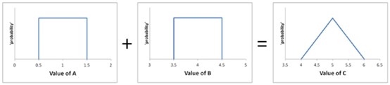
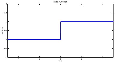
Let’s say you need to add these two rectangle functions. Would you guess that the result would be a triangle? If you looked carefully at the x-axis for each, you might. Otherwise, you would expect another rectangle. The simulation would not be fooled.

Another of Sam’s examples exactly represents the flaw of averages. He postulates a river that is forecast to crest 50 feet. Protecting the town are 50 ft. dikes. No problem, right? That is until you look at the range for the forecast. Turns out, it is even money for 45 ft., no problem, and 55 ft., $2 billion problem. The damage from the average crest of 50 feet is zero. However, the average damage is $1 billion, the average of $0 and $2 billion. In the real world, the spread would be greater and the probabilities lumpier, but this simple example makes the point for simulation rather than quick observation.

At this point, you may be thinking that you have heard of Monte Carlo  simulation, but doesn’t it get a bad rap? Has it not been debunked? I would not agree with either statement. Here is a couple reasons why its reputation may be less than sterling. The first is that if you build a bad model or incomplete spreadsheet, it does not matter what add-ins you utilize. Monte Carlo rides on your spreadsheet.

The second could be a misunderstanding of what Monte Carlo does. This may be clear after we review the process:

• Build the spreadsheet without Monte Carlo.
• Substitute a probability distribution for any factor that has inherent or situational uncertainty.
• The spreadsheet calculates results perhaps thousands of times, each time using a different set of random values based on the probability functions.
• Output includes distributions of possible outcomes.

I have heard people question the benefit of running the spreadsheet multiple times. Wouldn’t you keep getting the same answer? You would not because each run will substitute a different number for every cell that has a function. Those input numbers are not totally random nor equally likely. Their frequency directly correlates to the function in the cell. Thus, you generate an output with these features:

• Probabilistic Results: Results show not only what could happen, but how likely each outcome is.
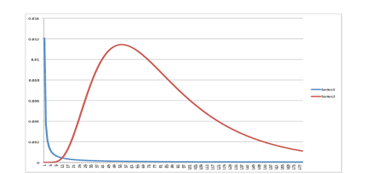
• Graphical Results:
  • Curve
  • Histogram
  • Cumulative probability distribution
• Sensitivity Analysis: See which inputs had the biggest effect on results.
• Scenario Analysis: See exactly which inputs worked together when certain outcomes occurred.

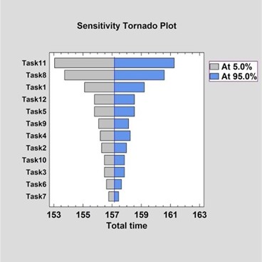
The two output charts that should be most useful for valuation analysis are the cumulative probability, shown here, and the sensitivity, also known as the tornado chart.

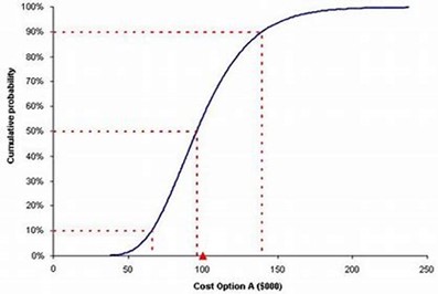
This example shows the chance that a part could be developed at or below a certain price. One could observe that there is a 50/50 chance of coming in less than 95. There is a 90% chance of staying below 140. Armed with this visual data, a company could decide whether to proceed with development; considering probabilities and budget constraints. No single number or set of a few spreadsheet runs will offer this much information.

The sensitivity chart, shown here, helps to determine which inputs or assumptions need to be tweaked or altered to improve the results. It is rarely as perfect a tornado ploy shape, as this example illustrates, but can still be an eye opener.

There are several Monte Carlo products that work seamlessly with Excel, and possibly other spreadsheet programs. You install them as an add-in, then invoke the various functions in a similar manner to built-in functions. The offerings differ in price, ease of use, support, and sophistication of the probability distributions. The information in this article should apply to any of them.

To create the Monte Carlo spreadsheet, be sure to model the effects we have reviewed thus far. The hurdle rate should reflect possibly higher interest rates than in previous years due to inflation and higher interest rate uncertainty. Be careful because the perceived rate may be unnecessarily high. Those higher actual and perceived rates may cause investment to be reduced both for textbook reasons and fear of making a mistake. We like to assume rational corporate actors who will always invest where the likely return exceeds the cost of capital. The agency problem and human nature variable temper that view. There are studies linking volatile costs of capital to overly conservative investment regimes.

Forecasting free cash can be challenging for the usual reasons and exacerbated by the effects of inflation on sales. The nominal value of each sale can respond to inflation, yet total units can reduce. It depends at least partly on the elasticity of demand. Yet, many companies do not pay a lot of attention to their demand curve. Thus, the profit and hence the free cash generated from each sale might require further study.

Set up your NPV, EVA, or IRR spreadsheet the usual way. Replace the hurdle rate with a probability function. Likewise, consider too that free cash flow and drivers of free cash that might also be affected by volatile rates or inflation. While the purist in me would like to see a perfect granular equation for each of those cells, you can get most of the benefit keeping it relatively simple. Stick to normal, log-normal, step, and diagonal distributions. They do not require a PhD in statistics and your audience will grasp the concepts.

The hurdle rate should be log-normal, in keeping with the analysis from the differential equations. You still have to select the median and standard deviation. There is enough historical and trend data to get a reasonable result. You can choose a different hurdle rate function for each year of your spreadsheet, but I do not recommend it. You might introduce more heat than light.

Modeling the probabilities for free cash and its components could be more difficult than for the hurdle rate and is likely to be company specific. Observing past behavior as well as interviewing decision makers should help. We can always update our models as we develop more insight or as the passage of time reveals our forecasting accuracy.

If your valuation calculation depends on risky projects, explicitly include risk in cash flow forecasts. Do not increase the hurdle rate. Results are very sensitive to small interest changes. You could also be hiding opaque risk assumptions.

The first output you want to specify is the cumulative probability distribution. Consider this example:

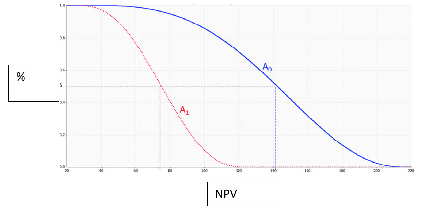
Company A₀ has a higher expected NPV than company A₁ at every level of probability, either because of different assumptions or being a better firm. Based on assumptions of risk or confidence of completion, you would not only value A₀ higher, but you would also see graphically what NPV you were comfortable supporting. Most likely, so would anyone you showed this to.

If you were not happy with the results, or you just wanted to see the effects of various tweaks, review the tornado chart. Then change the spreadsheet cells that will have the greatest impact on the outcome.

Clearly, there is a lot of art and science to selecting the best probability function and choosing the most appropriate coefficients. The good news is that all the machinations occur inside your spreadsheet. Changes are easy to implement, and the effects are immediate. You can benefit from the research that created the differential equations without having to directly solve any of them.

Best of all, we have a methodology to deal with variable interest rates. We are not striving for perfect models. Approximately right beats precisely wrong.

---

Alan E. Gorlick is CEO of Gorlick Financial Strategies, in Venice, Florida. He has been a part-time college professor since 1989, teaching MBA and undergraduate finance, economics, and accounting; securities and investment advisory services offered through NEXT Financial Group, Inc.; and member FINRA/SIPC. Gorlick Financial Strategies is not an affiliate of NEXT Financial Group.

Mr. Gorlick can be contacted at (941) 303-6921 or by e-mail to alan@gorlickfinancialstrategies.com.