Accepting and Rejecting Data from Public Company Data
Valuation analysts who, for whatever reason, eschew the publicly traded guideline company method but who would like to use option models for various aspects of the valuation assignment, face a conundrum. All option models require, as an input, a volatility factor in percentage format. Since the only place to derive such a volatility factor (usually defined as the standard deviation of total returns) is from public company data, how do you reject public company data on the one hand over here but use it on the other hand over there? Using non-public subject company data and standard valuation techniques, the authors offer two solutions to this problem.
[su_pullquote align=”right”]Resources:
Discounts for Lack of Marketability (DLOM) Workshop
Working Your Way Through the DLOM Minefield
Review of Option-based Models for Discount for Lack of Marketability
The Three Valuation Approaches—Challenges and Issues
[/su_pullquote]
Valuation analysts who, for whatever reason, eschew the publicly traded guideline company method but who would like to use option models for various aspects of the valuation assignment, face a conundrum. All option models require, as an input, a volatility factor in percentage format. Since the only place to derive such a volatility factor (usually defined as the standard deviation of total returns) is from public company data, how do you reject public company data on the one hand over here but use it on the other hand over there? Using non-public subject company data and standard valuation techniques, the authors offer two solutions to this problem.
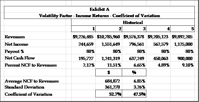
Our first solution is an indirect method and is shown on Exhibit A, where we define the volatility factor as the coefficient of variation. Our example is for only five years, but we suggest that you use as many years of data as available. We calculate the coefficient of variation by dividing the standard deviation by the mean, and you are free to use either dollars or percentages in the equation. Inserting the calculated volatility factors into the Longstaff DLOM model with a lockout period of five years returns DLOMs of 57.3% and 47.5% for the dollar and percentage figures, respectively. For those valuation analysts who feel that this method is a poor substitute for the standard deviation of total returns, we offer a second solution.
This solution is more complicated than the first, but should be recognizable as the Gordon Growth Model dressed up in Monte Carlo simulation style in order to produce a standard deviation of total returns, i.e., a volatility factor expressed directly in percentage terms. While we have chosen a single period capitalization model for the sake of simplicity of both use and presentation, a more complex multi-period discounted cash flow model will also work.
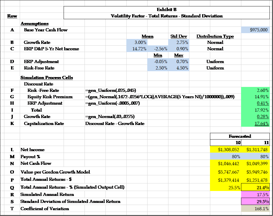
Total returns consist of the current year’s dividends plus capital gains or losses calculated as the difference between beginning of year and end of year market value. We use the Gordon Growth Model to develop capital gains or losses and then add that result to the current year’s expected cash pay-out. This sum of total returns is then divided by the average of beginning and ending market values to give us a total return for the year expressed as a percentage. In turn, the cell that contains the total percentage return for the year is the cell we have chosen to be the output cell for our Monte Carlo simulation. Our simulation software, XLSim, will produce the average total return and the standard deviation of that average for the 1,000 trials we have selected.
Using the assumptions to develop the simulating process cells shown on Exhibit B along with the XLSim formula for the distribution formula chosen, our simulated output cells are 17.5% for the average of total annual returns and 29.5% for the standard deviation of that average total annual return. Inserting the 29.5% standard deviation of total returns into the Longstaff DLOM model gives us a DLOM of 39.2%. Of course, your subject company outputs will differ, as these results are to the ranges of variability in the input data. A company with volatile cash flows, growth rates and risk factors will have higher or lower standard deviations and coefficients of variation.
To correctly interpret the data shown on Exhibit B, understand that rows A–E are fixed assumptions, along with row M, and are color-coded light blue. Rows F–K, color-coded light green, are simulating process cells or cells that result from being operated on by a process cell and can vary infinitely each time the F9 key is activated. Rows L, N, O, P, and Q, color-coded yellow, are calculating cells derived from the interactions of the process cells with the structure of the Gordon Growth Model as described above. These rows too can vary infinitely upon activation of the F9 key. Rows R and S, color-coded pink, are simulation output rows produced by the XLSim software. These rows are fixed output and do not vary. Row T, color-coded gray, is derived by dividing row S by row R. Therefore, when reviewing Exhibit B, keep in mind that what you are looking at for the most part is just one snapshot of an infinite number of possible inputs, processes, and output scenarios. Only rows R, S, and T have any concrete meaning—the rest is all calculation setup material.
Without considering the question of whether the total returns for small, privately-held companies ought to be more volatile than larger, publicly traded companies, let us look at some historical data from the public market contained in Exhibit C. The upper half of Exhibit C shows statistics for total returns, both for the periods 1926–2016 and 1963–2016. Both our simulated standard deviation of 29.5% and coefficient of variation of 168.1% shown on Exhibit B fall in the ranges of 24.3%–31.0% for standard deviation and 158.2%–193.0% for coefficient of variation.
The lower half of Exhibit C shows statistics for income returns only for the same two periods. Both coefficients of variation of income returns shown on Exhibit A of 47.5% and 52.7% almost fall within the range shown on Exhibit C of 48.6%–53.1%.
Are we onto something here?
[divide] Mark G. Filler, CPA, ABV, CVA, AM, CBA leads Filler & Associates’ Litigation and Claims Support practice in Portland, Maine.
He has been in public accounting since February 1968. Mr. Filler has been a Certified Public Accountant since November 1972, a Certified Valuation Analyst since November 1994, a Certified Business Appraiser since May 1997, Accredited in Business Valuation since January 1999, and an Accredited Member since April 2004.
His experience has been entirely with small firms, and his focus has been on helping small business entrepreneurs solve their tax and business problems. His services include aid and advice around tax minimization, business planning and major business decisions, financing, determining management information needs, setting up cash management tools, instituting cost reduction and budgeting techniques, and the placement of bookkeepers and controllers.
Mr. Filler can be contacted at (207) 591-6424 or by e-mail to mfiller@filler.com.
Edward Giardina, MSA, CPA, ABV, CVA, is a partner with Giardina & French, CPAs in Boston, Massachusetts, a tax boutique firm. Mr. Giardina specializes in business valuation for estate and gift tax, and for shareholder transactions. He has presented at the NACVA and the CTI’s Annual Consultants’ Conference and frequently at its Massachusetts chapter, which he helped organize and run for the past 23 years. Mr. Giardina is especially well-known for his contribution to the S corporation valuation controversary following the Tax Court decision in the Gross case.
Mr. Giardina can be contacted at (617) 720-5520 or by e-mail to EGiardina@giardinafrench.com.


